Iterative Classroom Teaching

(1)

The Thirty-Third AAAI Conference on Artificial Intelligence (AAAI-19)

Iterative Classroom Teaching

Teresa Yeo

LIONS, EPFL [email protected]

Parameswaran Kamalaruban

LIONS, EPFL

[email protected]

Louis Faucon

Pierre Dillenbourg

Volkan Cevher

LIONS, EPFL [email protected]

Abstract

We consider the machine teaching problem in a classroom-like setting wherein the teacher has to deliver the same examples to a diverse group of students. Their diversity stems from dif-ferences in their initial internal states as well as their learning rates. We prove that a teacher with full knowledge about the learning dynamics of the students can teach a target concept to the entire classroom usingO min{d, N}log1

exam-ples, wheredis the ambient dimension of the problem,Nis the number of learners, andis the accuracy parameter. We show the robustness of our teaching strategy when the teacher has limited knowledge of the learners’ internal dynamics as provided by a noisy oracle. Further, we study the trade-off be-tween the learners’ workload and the teacher’s cost in teaching the target concept. Our experiments validate our theoretical results and suggest that appropriately partitioning the class-room into homogenous groups provides a balance between these two objectives.

Introduction

Machine teaching considers the inverse problem of machine learning. Given a learning model and a target, the teacher aims to find an optimal set of training examples for the learner (Zhu et al. 2018; Liu et al. 2017). Machine teach-ing provides a rigorous formalism for various real-world applications such as personalized education and intelligent tutoring systems (Rafferty et al. 2016; Patil et al. 2014), imita-tion learning (Cakmak and Lopes 2012; Haug, Tschiatschek, and Singla 2018), program synthesis (Mayer, Hamza, and Kuncak 2017), adversarial machine learning (Mei and Zhu 2015), and human-in-the-loop systems (Singla et al. 2014; 2013).1

Individual teaching Most of the research in this domain thus far, has focused on teaching a single student in the batch setting. Here, the teacher constructs an optimal training set (e.g., of minimum size) for a fixed learning model and a tar-get concept and gives it to the student in a single interaction (Goldman and Kearns 1995; Zilles et al. 2011; Zhu 2013; Doliwa et al. 2014). Recently, there has been interest in study-ing the interactive settstudy-ing (Liu et al. 2017; Zhu et al. 2018; Chen et al. 2018; Hunziker et al. 2018), wherein the teacher

1

http://teaching-machines.cc/nips2017/

focuses on finding an optimal sequence of examples to meet the needs of the student under consideration, which is, in fact, the natural expectation in a personalized teaching environ-ment (Koedinger et al. 1997). (Liu et al. 2017) introduced the iterative machine teaching setting wherein the teacher has full knowledge of the internal state of the student at every time step using which she designs the subsequent optimal example. They show that such an “omniscient” teacher can help a single student approximately learn the target concept usingO log1training examples (whereis the accuracy parameter) as compared toO 1

examples chosen randomly by the stochastic gradient descent (SGD) teacher.

Classroom teaching In real-world classrooms, the teacher is restricted to providing the same examples to a large class of academically-diverse students. Customizing a teaching strategy for a specific student may not guarantee optimal performance of the entire class. Alternatively, teachers may constitute a partitioning of the students so as to maximize intra-group homogeneity while balancing the orchestration costs of managing parallel activities. (Zhu, Liu, and Lopes 2017) propose methods for explicitly constructing a mini-mal training set for teaching a class of batch learners based on a minimax teaching criterion. They also study optimal class partitioning based on prior distributions of the learners. However, they do not consider an interactive teaching setting.

Overview of our Approach

In this paper, we study the problem of designing optimal teaching examples for a classroom of iterative learners. We refer to this new paradigm asiterative classroom teaching

(CT). We focus on online projected gradient descent learners under squared loss function. The learning dynamics com-prise of the learning rates and the initial states which are different for different students. At each time step, the teacher constructs the next training example based on information regarding the students’ learning dynamics. We focus on the following teaching objectives motivated by real-world class-room settings, where at the end of the teaching process:

(i) all learners in the class converge to the target model (cf.

Eq. (1)),

(ii) the class on average converges to the target model (cf.

(2)

(a) A Nao robot writing on a digital tablet.

(b) Example of five interactions for writing the word ”nao”. The top row shows the writing of the robot, the bottom row shows the child’s writing.

Figure 1: The robot writes iteratively adapted to the handwriting profile of the child; if the child’s handwriting is shaky, the robot too writes with a shaky handwriting. In correcting the robot’s handwriting, the child works towards remediating theirs.

Contributions We first consider that setting wherein at all times, the teacher has complete knowledge of the learning rates, loss function, and full observability of the internal states of all the students in the class. A naive approach here would be to apply (Liu et al. 2017)’s omniscient teaching strategy individually for each student in the class. This would require

O Nlog1

teaching examples, whereNis the number of students in the classroom. We present a teaching strategy that can achieve a convergence rate ofO klog1

, where

kis the rank of the subspace in which the students of the classroom lie (i.e.k≤min{d, N}, wheredis the ambient dimension of the problem). We also prove the robustness of our algorithm in noisy and incomplete information settings. We then explore the idea of partitioning the classroom into smaller groups of homogenous students based on either their learning ability or prior knowledge. We also validate our theoretical results on a simulated classroom of learners and demonstrate their practical applications to the task of teaching how to classify between butterflies and moths. Further, we show the applicability of our teaching strategy to the task of teaching children how to write (cf. Figure 1).

The Model

In this section, we consider a stylized model to derive a solid understanding for the dynamics of the learners. This simplicity of our model will then allow us to gain insights into classroom partitioning (i.e., how to create classrooms), and then explore the key trade-offs between the learners’ workload as well as the teacher’s orchestration costs. By orchestration costs, we mean the number of examples the teacher needs to teach the class.

Notation Define{ai}N_i₌₁:={a1, . . . , aN}as a set ofN el-ements and[N] :={1, . . . , N}as the index set. For a given matrixA, denoteλi(A)and ei(A) to be the i-th largest eigenvalue ofAand the corresponding eigenvector respec-tively.k·kdenotes the Euclidean norm unless otherwise spec-ified. The projection operation on a setWfor any elementy

is defined as follows:

Proj_W(y) := arg min

x∈W

kx−yk2

Parameters In synthesis-based teaching (Liu et

al. 2017), X =

x∈_Rd_,_k_x_{k ≤}_D

X represents

the feature space and the label set is given by

Y = R(for regression) or{1,2, . . . , m}(for classification).

A training example is denoted by (x, y) ∈ X × Y.

Further, we define the feasible hypothesis space by

W =

w∈_Rd_,_k_w_{k ≤}_D

W , and denote the target

hypothesis byw∗.

Classroom The classroom consists ofN students. Each studentj∈[N]has two internal parameters: i) the learning rate (at timet) represented byηt

j, and ii) the initial internal state given byw0

j ∈ W. At each time stept, the classroom receives a labelled training example(xt_{, y}t₎_{∈ X × Y}_and each studentjperforms a projected gradient descent step as follows:

wt+1

j = ProjW wtj−η t j

∂` π(wt j, xt), yt

∂wt j

!

,

where ` is the loss function and π(wt

j, xt) is the stu-dent’s label for example xt_{. We restrict our analysis to} the linear regression case whereπ(wt

j, xt) =

wt j, xt

and

`

wt j, xt

, yt

=1

2

wt j, xt

−yt2 .

Teacher The teacher, over a series of iterations, interacts with the students in the classroom and guides them towards the target hypothesis by choosing “helpful” training examples. The choice of the training example depends on how much information she has about the students’ learning dynamics.

• Observability: This represents the information that the teacher possesses about the internal state of each student. We study two cases: i) when the teacher knows the ex-act value

wt j

N

j=1, and ii) when the teacher has a noisy

estimate denoted byw˜t j

N

j=1at any timet.

(3)

normal distribution at every time step, while the teacher only has access to the past values.

Teaching objective In the abstract machine teaching set-ting, the objective corresponds to approximately training a predictor. Given an accuracy valueas input, at timeT we say that a studentj∈[N]has approximately learnt the

tar-get conceptw∗ _when

wT_j −w∗

≤. In the strict sense, the teacher’s goal may be to ensure that every student in the classroom converges to the target as quickly as possible, i.e.,

wT_j −w∗

≤ ,∀j∈[N]. (1) The teacher’s goal in the average case however, is to ensure that the classroom as a whole converges tow∗_{in a minimum} number of interactions. More formally, the aim is to find the smallest valueT such that the following condition holds:

1 N N X i=1

wT_j −w∗

2

≤ . (2)

Classroom Teaching

We study the omniscient and synthesis-based teacher, equiv-alent to the one considered in (Liu et al. 2017), but for the iterative classroom teaching problem under the squared loss given by`(hw, xi, y) := ₂1(hw, xi −y)2. Here the teacher has full knowledge of the target conceptw∗, learning rates

{ηj} N

j=1(assumed constant), and internal states

wt j

N j=1of

all the students in the classroom.

Teaching protocol At every time stept, the teacher uses all the information she has to choose a training examplext_{∈ X} and the corresponding labelyt₌_h_w_∗_{, x}t_{i ∈ Y} _{(for linear} regression). The idea is to pick the example which minimizes the average distance between the students’ internal states and the target hypothesis at every time step. Formally,

xt_{= arg min} x∈X 1 N N X j=1 wt j−ηj

∂`Dwt j, x

E

,hw∗_{, x}_i

∂wt j

−w∗ 2 .

Note that constructing the optimal example at timet, is in general a non-convex optimization problem. For the squared loss function, we present a closed-form solution below.

Example construction Define,wˆt

j := wjt−w∗, forj ∈

[N]. Then the teacher constructs the common example for the whole classroom at timetas follows:

1. the feature vectorxt₌_γ

txˆtsuch that (a) the magnitudeγt:

γt≤DX, and2−ηjγt2 ≥ 0,∀j∈[N]. (3) (b) the directionxˆt_(with_k_x_ˆt_k_{= 1}_):

ˆ

xt := arg max

x:kxk=1

x>Wtx = e1 Wt

, (4)

where

αt

j := ηjγt2 2−ηjγ2t

(5)

Wt _:= 1

N

N X

j=1

αt jwˆ

t j wˆ

t j

>

. (6)

Algorithm 1CT: Classroom teaching algorithm

Input:targetw∗∈ W; students’ learning rates{ηj} N j=1

Goal:accuracy

Initializet= 0

Observew0

j N

j=1

while _N1 PN j=1

w_jt−w∗

2

> do

Observewt j

N j=1

Chooseγts.t.γt≤DX, and2−ηjγt2≥0,∀j∈[N] ConstructWt_{given by Eq. (6)}

Pick examplext₌_γ

t·e1(Wt)andyt=hw∗, xti

Provide the labeled example(xt_{, y}t₎_{to the classroom} Students’ update:∀j ∈[N],

wjt+1←ProjW wtj−ηj

wtj, x t

−yt

xt

. t←t+ 1

end while

2. the labelyt₌_h_w∗_{, x}t_i_.

Algorithm 1 puts together our omniscient classroom teach-ing strategy. Theorem 1 provides the number of examples required to teach the target concept.2

Theorem 1. Consider the teaching strategy given in Algorithm 1. Let k := maxt{rank (Wt)}, where Wt is

given by Eq.(6). Defineαj := mintαjt,αmin:= mint,jαtj,

and αmax := maxt,jαjt, where αtj is given by Eq. (5).

Then after t = O

log₁ 1

−αmin

k −1

log1

rounds, we

have _N1 PN j=1

w_jt−w∗

2

≤ . Furthermore, after t =

O

max

log₁₋1_αj− 1

log1,log₁ 1

−αmin

k −1

log1

rounds, we havewt_j−w∗

2

≤,∀j∈[N].

Remark 1. By using the fact thatexp (−2x)≤log (1−x), for 2x ≤ 1.59, we can show that for k ≥ 2αmin

1.59 ,

O

log₁ 1

−αmin

k −1

log1

≈ O k αminlog

1

.

Based on Theorem 1 and Remark 1, note that the teaching strategy given in Algorithm 1 converges in O klog1 samples, where k = maxt{rank (Wt)} ≤ min{d, N}. This is in fact a significant improvement (especially when

N d) over the sample complexity O Nlog1

of a teaching strategy which constructs personalized training examples for each student in the classroom.

Choice of magnitudeγt We consider the following two choices ofγt:

1. staticγt= min n

1

maxj∈[N]√ηj, DX

o

: This ensures that the classroom can converge without being partitioned into

2

(4)

small groups of students. However, the valueαmin

be-comes small and as a result, the sample complexity in-creases.

2. dynamic γt = min

rPN

j=1ηjkwtj−w∗k 2

PN

j=1η2jkwtj−w∗k

2, D_X

: This

provides an optimal constant for the sample complexity, but requires that for effective teaching the classroom is par-titioned appropriately. This value ofγtis obtained by max-imizing the termPN

j=1ηjγ2t 2−ηjγt2 wt_j−w∗

2

.

Natural partitioning based on learning rates In order to satisfy the requirements given in Eq. (3), for every student

j∈[N], we require (for dynamicγt):

ηjγt2 ≤ ηmax PN

j=1ηj

w_jt−w∗

2

PN j=1η

2

j

wt_j−w∗

2

≤ ηmax

PN j=1ηj

w_jt−w∗

2

ηminPN j=1ηj

wt_j−w∗

2 ≤ 2, (7)

where ηmax = maxjηj, and ηmin = minjηj. That is, if

ηmax ≤2ηmin, we can safely use the above optimalγt. This observation also suggests a natural partitioning of the class-room: {[ηmin,2ηmin),[2ηmin,4ηmin), . . . ,[2m_ηmin,₂_ηmax₎_}_, wherem=jlog₂ηmax

ηmin k

.

Robust Classroom Teaching

In this section, we study the robustness of our teaching strat-egy in cases when the teacher can access the current state of the classroom only through a noisy oracle, or when the learning rates of the students vary with time.

Noise in

w

t j

’s

Here, we consider the setting where the teacher cannot di-rectly observe the students’ internal states

wt j

N

j=1,∀tbut

has full knowledge of students’ learning rates{ηj} N j=1.

De-fine αmin := mint,jαtj, and αavg := maxt_N1 PN_j₌₁αtj,

whereαt

jis given by Eq. (5). At every time stept, the teacher only observes a noisy estimate ofwt

j(for eachj∈[N]) given by

˜

wt j := w

t j+δ

t

j, (8)

where δt

j is a random noise vector such that

δt_j

≤

4_ααavg

mind+1

DW

. Then the teacher constructs the example

as follows:

ˆ

xt _{:= arg max}

x:_kx_k=1

x>    1 N N X j=1 αt jwˆ

t j wˆ

t j >    x

xt _:= _γ

txˆtandyt=w∗, xt, (9) wherewˆt

j := ˜wtj−w∗, andγtsatisfies the condition given in Eq. (3). The following theorem shows that even under this noisy observation setting Eq. (8), with the example construc-tion strategy described in Eq. (9), the teacher can teach the classroom with linear convergence.

Theorem 2. Consider the noisy observation setting given by Eq. (8). Let k := maxt{rank (Wt)} where

Wt ₌ 1

N PN

j=1α

t j w˜

t j−w∗

˜

wt j−w∗

>

. Then for the robust teaching strategy given by Eq. (9),

af-ter t = O

log₁ 1

−αmin

k −1

log1

rounds, we have

1

N PN

j=1

wt_j−w∗

2

≤.

Noise in

η

t j

Here, we consider a classroom of online projected gradient descent learners with learning ratesηt

j N

j=1, whereη

t j ∼

N(ηj, σ). We assume that the teacher knows σ(which is constant across all the students) and{ηj}

N

j=1, but doesn’t

knowηt j

N

j=1. Further, we assume that the teacher has full

observability ofwt j

N

j=1. At timet, the teacher has access to

the historyHt :=

ws j

t

s=1,

ηs j

t−1

s=1:∀j ∈[N]

. Then

the teacher constructs the example as follows (depending only onHt):

ˆ

xt _{:= arg max}

x:kxk=1

x>W¯t_x ₌ _e

1 W¯t

xt _:= _γ

txˆtandyt=

w∗, xt

, (10)

where

γ2

t ≤

2ηj

σ2₊_η2

j

,∀j∈[N] (11)

¯

ηt j :=

1

t−1

X s=1 ηs j (12) ¯ αt j := 2γ

2

tη¯ t j−γ

4

t

t−2

t−1σ 2_{+ ¯}_ηt

j 2

(13)

ˆ

wtj := w t

j−w∗and (14)

¯

Wt _:= 1

N N X j=1 ¯ αt jwˆjt wˆtj

>

. (15)

The following theorem shows that, in this setting, the teacher can teach the classroom in expectation with linear conver-gence.

Theorem 3. Let k := maxt

rank W¯t _where _W_¯t _is

given by Eq.(15). Defineα¯min := mint,jα¯tj, andβmin :=

minj,t

αt_j

¯

αt j

, whereαt j:= 2γ

2

tηj−γt4 σ2+η2j

andα¯t jgiven

by Eq.(13). Then for the teaching strategy given by Eq.(10),

aftert=O

log 1

1−βmin ¯αmin

k

−1

log1

!

rounds, we have

E h 1 N PN j=1

w_jt−w∗

2i

≤.

Classroom Partitioning

(5)

1 2 3

4 5

6 6

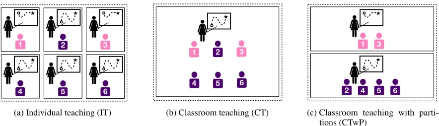
(a) Individual teaching (IT)

1 2 3

4 5 6

(b) Classroom teaching (CT)

1 3

2 4 5 6

(c) Classroom teaching with parti-tions (CTwP)

Figure 2: Comparisons between individual teaching (IT) and classroom teaching (CT and CTwP) paradigms.

the same time, classroom teaching increases the students’ workload substantially because it requires catering to the needs of academically diverse learners. We overcome these pitfalls by partitioning the given classroom ofN students intoKgroups such that the orchestration cost of the teacher and the workload of students is balanced. Figure 2 illustrates these three different teaching paradigms.

LetT(K)be the total number of examples required by the teacher to teach all the groups. Let S(K)be the average number of examples needed by a student to converge to the target. We study the total cost defined as:

cost(K) := T(K) +λ·S(K),

whereλquantifies the trade-off factor, and its value is ap-plication dependent. In particular, for any givenλ, we are interested in that valueKthat minimizescost(K). For ex-ample, whenλ=∞, the focus is on the student workload; thus the optimal teaching strategy is individual teaching,i.e.,

K=N. Likewise, whenλ= 0, the focus is on the orches-tration cost; thus the optimal teaching strategy is classroom teaching without partitioning, i.e.,K= 1. In this paper, we explore two homogeneous partitioning strategies: (a) based on learning rates of the students{ηj}

N

j=1, (b) based on prior

knowledge of the students

w0

j N

j=1.

Experiments

Teaching Linear Models with Synthetic Data

We first examine the performance of our teaching algorithms on simulated learners.

Setup We evaluate the following algorithms: (i) classroom teaching (CT) - the teacher gives an example to the en-tire class at each iteration, (ii) CT with optimal partitioning (CTwP-Opt) - the class is partitioned as defined in Section , (iii) CT with random partitioning (CTwP-Rand) - the class is randomly assigned to groups, and (iv) individual teaching (IT) - the teacher gives a tailored example to each student. An algorithm is said to converge when_N1 P

ikw t

i−w∗k22≤.

We set the number of learnersN = 300and accuracy param-eter= 0.1.

Average error and robustness of CT We first consider the noise free classroom setting withd= 25, learning rates be-tween[0.05,0.25], andDX = 2. The plot of the error over

time is shown in Figure 3a, together with the performance of four selected learners. Our algorithm exhibits linear con-vergence, as per Theorem 1. The slower the learners and the further away they are fromw∗_{, the longer they take to} converge. Figure 3d shows how convergence is affected as the noise level,δ, increases in the robust classroom teach-ing settteach-ing as described in Section . Although the number of iterations required for convergence increases, it is still significantly lower than the noise-free IT.

Convergence for classroom with diverseη We study the effect of partitioning byηon the performance of the algo-rithms described. The diversity of the classroom varies from 0 (where all learners in the classroom haveη = 0.1) to 0.5 (where for all learnersη∈[0.1,0.6]chosen randomly), and so on. Figure 3b and Figure 3c depict the number of iter-ations and number of examples needed by the teacher and students respectively to achieve convergence. As expected, IT performs best, and CTwP-Opt consistently outperforms CT. For a class with low diversity, partitioning is costly. How-ever as diversity increases, partitioning is beneficial from the teachers’ perspective. Note that the dip at a diversity of 0.15 for both plots is due to the value ofD_X. For the staticγt, withDX = 2, all learners with rates less than 0.25 will be negatively affected. As the minimum value ofη is 0.1, at zero diversity, all learners are affected the most. As diversity increases to 0.15, all learners are affected but to a lesser de-gree. Figure 3e shows how the optimal algorithm, the one that minimizes cost, changes withλand diversity ofη. When diversity is low and there is a low trade-off factor on the students’ workload, CT performs best. At high values, IT has the lowest cost. CTwP-Opt falls between these two regimes.

Convergence for classroom with diverse w0 _{Next, we}

(6)

0 100 200 300 400 500 Iteration

0 10 20 30 40 50 60

Error

= 0.05, w0 close

= 0.15, w0 close

= 0.05, w0 far

= 0.15, w0 far

Average

(a) Error plot for CT; average error of the classroom and the error of four selected learners.

0.0 0.5 1.0 1.5 2.0 2.5

Diversity of 0

500 1000 1500 2000 2500 3000

Teacher: Total number of iterations

CT CTwP-Opt CTwP-Rand IT

(b) Total iterations needed for conver-gence from the teacher’s perspective.

0.0 0.5 1.0 1.5 2.0 2.5

Diversity of 0

50 100 150 200 250 300 350 400

Students: Average number of iterations

(c) Total iterations per student needed for convergence from the students’ per-spective.

2200 2250 2300

IT, || || = 0

0 5 10 15 20

|| || 150

200 250

CT CT, || || = 0

(d) Total iterations needed for conver-gence in noisywtcase as the noise,δ,

increases.

0.0 0.5 1.0 1.5 2.0 2.5 Diversity of

0 4 8 12 16

: T

ea

ch

er

/st

ud

en

ts

co

st

tra

de

of

f CT CTwP-Opt IT

(e)λ: Trade-off between teacher’s and students’ cost with increasingη diver-sity.

1 2 3 4 5 6 7 8 9 10 Diversity of w0

0 20 40 60 80 100

: T

ea

ch

er

/st

ud

en

ts

co

st

tra

de

of

f CT CTwP-Opt IT

(f)λ: Trade-off between teacher’s and stu-dents’ cost with increasingw0 diver-sity.

Figure 3: (3a) and (3d) show the convergence results for the noise-free and noisy settings. CT is robust and exhibits linear convergence. (3b), (3c) and (3e) show the convergence results and trade-off for a classroom with diverseη. (3f) shows the trade-off for a classroom with diversew0_.

increase. The results are the same as withηpartitioning and CTwP-Opt outperforms in most regimes.

Teaching How to Classify Butterflies and Moths

We now demonstrate the performance of our teaching algo-rithms on a binary image classification task for identifying insect species, a prototypical task in crowdsourcing applica-tions and an important component in citizen science projects such as eBird (Sullivan et al. 2009).

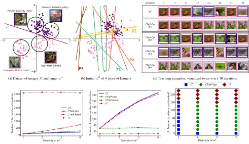
Images and Euclidean embedding We use a collection of 160 images (40 each) of four species of insects, namely (a) Caterpillar Moth (cmoth), (b) Tiger Moth (tmoth), (c) Ringlet Butterfly (rbfly), and (d) Peacock Butterfly (pbfly), to form the teaching setX. Given an image, the task is to classify if it is a butterfly or a moth. However, we need a Euclidean embedding of these images so that they can be used by a teaching algorithm. Based on the data collected by (Singla et al. 2014), we obtained binary labels (whether a given image is a butterfly or not) forX from a set of 67 workers from Amazon Mechanical Turk. Using this annotation data, the Bayesian inference algorithm of (Welinder et al. 2010) allows us to obtain an embedding, shown in Figure 4a, along with the targetw∗(the best fitted linear hypothesis forX).

Learners’ hypotheses The process described above to ob-tain the embedding in Figure 4a simultaneously generates an embedding of each of the67annotators as linear

hypothe-ses in the same 2D space. Termed as “schools of thought” by (Welinder et al. 2010), these hypotheses capture various real-world idiosyncrasies in the AMT workers’ annotation behavior. For our experiments, we identified four types of learners’ hypotheses; those who (i)misclassify tmoth as but-terfly (P1), (ii)misclassify rbfly as moth (P2), (iii)misclassify pbfly as moth (P3)and (iv)misclassify tmoth and cmoth as butterflies. Figure 4b shows an embedding of three distinct hypotheses each of the four types of learners.

Creating the classroom We denote the hypotheses de-scribed above as initial statesw0 _{of the learners/students.}

Due to sparsity of data, we create a supersample of size60

for the four types of learners by adding a small noise. We set the classroom sizeN = 60. The diversity of the class, defined by the number of different types of learners present, varies from 1 to 4. Thus, diversity of1refers to the case when all60learners are of same type (randomly picked from P1, P2, P3, or P4), and diversity of4refers to the case when there are15learners of each type. We set a constant learning rate ofη = 0.05for all students.

(7)

Tiger Moth (tmoth)

Caterpillar Moth (cmoth) Ringlet Butterfly (rbfly)

Peacock Butterfly (pbfly)

w⇤

(a) Dataset of imagesXand targetw∗

P3

P4 _P1

P2

(b) Initialw0of 4 types of learners

CTwP-Opt (P1)

CT

1 2 11 12 21 22 31 32

Iterations

CTwP-Opt (P2)

CTwP-Opt (P3)

CTwP-Opt (P4)

(c) Teaching examples, visualized twice every 10 iterations.

1 2 3 4

Diversity of w0

0 500 1000 1500 2000 2500 3000

(d) Total iterations needed for convergence from the teacher’s perspective

1 2 3 4

Diversity of w0

60 80 100 120 140 160 180

Students: Average number of iterations

(e) Total iterations needed for convergence from the student’s perspective

1 2 3 4

Diversity of w0

0 40 80 120 160 200

: T

ea

ch

er

/st

ud

en

ts

co

st

tra

de

of

f

CT CTwP-Opt IT

(f)λ: Trade-off between teacher’s and students’ cost with increasingw0diversity

Figure 4: (4a) shows a low-dimensional embedding of the dataset and the target concept. (4b) shows an embedding of the initial states of three learners of each of the 4 types. (4c) are training examples selected by CT and CTwP-Opt teachers when the class has diversity 4. (4d) and (4e) show the number of iterations required to achieve-convergence from the teacher and student perspectives. (4f) shows how the optimal algorithm changes as we vary the trade-off parameterλ, and diversity of the class.

converged when _N1 P

ikw t i−w∗k

2

2≤.

Teaching examples Figure 4c consists of 5 rows of 20 thumbnail images each, depicting the training examples cho-sen in an actual run of the experiment when the diversity of the classroom is 4. The first row corresponds to the images chosen by CT. For instance, in iteration 1, CT chooses a tmoth example. While this example is most helpful for learners in P1 (confusing tmoths as butterflies), however, learners in P2 and P3 would have benefited more from seeing examples of butterflies. This increases the workload for the learners. The next four rows in Figure 4c correspond to the images chosen by CTwP-Opt when teaching partitions P1, P2, P3, and P4 respectively—these thumbnails show the personal-ized effect given the homogeneity of these partitions. For instance, for P1, the CTwP-Opt focuses on choosing tmoth examples thereby allowing these learners to converge faster while ensuring that the cost for learners in other partitions does not increase.

Convergence Figure 4d compares the performances of the teachers in terms of the total number of iterations required for convergence. CT performs optimally because every example chosen is provided to the entire class; CTwP-Opt requires only a few examples more, given the homogeneity of the partition and the partitions being of equal size. IT constructs

individually tailored examples for each learner in the class. Thus the combined number of iterations is much higher in comparison.

Teacher/students cost trade-off On the other hand, Figure 4e depicts the average number of examples required by each learner to achieve convergence as a function of diversity. This represents the learning cost from the students’ persective. IT performs best because the teacher chooses personalized ex-amples for each learner. CTwP-Opt performs considerably better than CT. This happens because partitioning groups to-gether learners of the same type. Figure 4f represents optimal algorithm given the diversity of the class and the trade-off fac-torλas defined in Section . As diversity increases, CTwP-Opt outperforms the other teachers in terms of the total cost.

Teaching How to Write

(8)

(a) Shaky and distorted handwriting (b) Shaky and rotated handwriting (c) Rotated and distorted handwriting

Figure 5: (5a) to (5c) shows samples of children’s handwriting where two of the three defined features are poor and the third is good.

(a) Teaching examples for shaky and rotated handwriting

(b) Teaching examples for distorted and shaky handwriting

(c) Teaching examples for distorted and ro-tated handwriting

(d) Teaching examples for distorted, rotated, shaky handwriting

Figure 6: (6a) to (6d) shows the sequence of examples, visualized every other iteration, chosen by our algorithm for different initial hypothesis of the children.

esteem and increases their commitment to the task as they are given the role of the one who “knows and teaches” (Rohrbeck et al. 2003; Chase et al. 2009). In our experiments, a robot iteratively proposes a handwriting adapted to the handwriting profile of the child, that they try to correct (cf.Figure 1b). We now demonstrate the performance of our algorithm in choosing this sequence of examples.

Generating handwriting dynamics A LSTM is used to learn and generate handwriting dynamics (Graves 2013). It is trained on children’s handwriting data collected from 1014 children from 14 schools.3 In the extended version of this paper (Yeo et al. 2018), we showed that the pool of samples has to be rich enough for teaching to be effective.4_{As our}

generative model outputs a distribution, we can sample from it to get a diverse set of teaching examples. We analyze our results for a cursive “f”, similar results apply for the other letters.

Handwriting features Concise Evaluation Scale (BHK) (Hamstra-Bletz, DeBie, and Den Brinker 1987) is a standard handwriting test used in Europe to evaluate children’s hand-writing quality. We adopt features such as (i) distortion, (ii) rotation, (iii) shakiness, and label each generated sample with a score for each of these features.

Creating the classroom Given a child’s handwriting sam-ple, we estimate their initial hypothesis,w0by how well each

of the above features have been written, in a similar fashion to the scoring of samples. As most children fair poorly in two out of the three features, we selected and partitioned them according to the following three types of handwriting charac-teristics, substantial (i) shakiness and rotation, (ii) distortion

3

The model has 3 layers, 300 hidden units and outputs a 20 component bivariate Gaussian mixture and a Bernoulli variable indicating the end of the letter. Each child was asked to write, in cursive, the 26 letters of the alphabet and the 10 digits on a tablet.

4

The attained result is for the squared loss function, however, the analysis holds for other loss function.

and shakiness, and (iii) distortion and rotation. Original sam-ples of each are shown in Figures 5a to 5c. We set a constant learning rate for all learners.

Teaching examples Figures 6a to 6c shows the training examples chosen by CTwP-Opt and Figure 6d by our CT algorithm. Each of the synthesized handwriting samples are labelled as good or bad, based on the average of their nor-malized scores. We then run a classification algorithm on each partition and the entire class. This returns a sequence of examples that the robot would propose, for the children to correct. For children with handwriting that is shaky and rotated but not distorted, the sequence of examples chosen by our algorithm shows examples that are not distorted but progressively smoother and upright. Similarly, for children with handwriting that is distorted and shaky, the sequence of examples shown is upright with decreasing distortion and shakiness. We did not show the convergence plots as they have similar characteristics as those from the previous exper-iments.

Conclusion

We studied the problem of constructing an optimal teaching sequence for a classroom of online gradient descent learners. In general, this problem is non-convex, but for the squared loss, we presented and analyzed a teaching strategy with linear convergence. We achieved a sample complexity of

O min{d, N}log1

(9)

achieve a good trade-off between the learners’ workload and the teacher’s orchestration cost. The sequence of examples returned by our experiments are interpretable and they clearly demonstrate a significant potential in automation for robotics.

Acknowledgments.This work was supported in part by the Swiss National Science Foundation (SNSF) under grant num-ber 407540 167319, CR21I1 162757 and NCCR Robotics.

References

Cakmak, M., and Lopes, M. 2012. Algorithmic and human teaching of sequential decision tasks. InAAAI.

Chase, C. C.; Chin, D. B.; Oppezzo, M. A.; and Schwartz, D. L. 2009. Teachable agents and the prot´eg´e effect: Increas-ing the effort towards learnIncreas-ing.Journal of Science Education and Technology18(4):334–352.

Chen, Y.; Singla, A.; Mac Aodha, O.; Perona, P.; and Yue, Y. 2018. Understanding the role of adaptivity in machine teaching: The case of version space learners. InNIPS. Christensen, C. A. 2009. The critical role handwriting plays in the ability to produce high-quality written text. The SAGE handbook of writing development284–299.

Doliwa, T.; Fan, G.; Simon, H. U.; and Zilles, S. 2014. Re-cursive teaching dimension, vc-dimension and sample com-pression.Journal of Machine Learning Research15(1):3107– 3131.

Feder, K. P., and Majnemer, A. 2007. Handwriting de-velopment, competency, and intervention. Developmental Medicine & Child Neurology49(4):312–317.

Goldman, S. A., and Kearns, M. J. 1995. On the complex-ity of teaching. Journal of Computer and System Sciences

50(1):20–31.

Graves, A. 2013. Generating sequences with recurrent neural networks. arXiv preprint arXiv:1308.0850.

Hamstra-Bletz, L.; DeBie, J.; and Den Brinker, B. 1987. Concise evaluation scale for children’s handwriting. Lisse: Swets1.

Haug, L.; Tschiatschek, S.; and Singla, A. 2018. Teaching in-verse reinforcement learners via features and demonstrations. InNIPS.

Hunziker, A.; Chen, Y.; Mac Aodha, O.; Gomez-Rodriguez, M.; Krause, A.; Perona, P.; Yue, Y.; and Singla, A. 2018. Teaching multiple concepts to a forgetful learner. CoRR

abs/1805.08322.

Johal, W.; Jacq, A.; Paiva, A.; and Dillenbourg, P. 2016. Child-robot spatial arrangement in a learning by teaching activity. InRobot and Human Interactive Communication (RO-MAN), 2016 25th IEEE International Symposium on, 533–538. IEEE.

Koedinger, K. R.; Anderson, J. R.; Hadley, W. H.; and Mark, M. A. 1997. Intelligent tutoring goes to school in the big city.

International Journal of Artificial Intelligence in Education (IJAIED)8:30–43.

Liu, W.; Dai, B.; Humayun, A.; Tay, C.; Yu, C.; Smith, L. B.; Rehg, J. M.; and Song, L. 2017. Iterative machine teaching. InICML, 2149–2158.

Mayer, M.; Hamza, J.; and Kuncak, V. 2017. Proactive synthesis of recursive tree-to-string functions from examples (artifact). InDARTS-Dagstuhl Artifacts Series, volume 3. Mei, S., and Zhu, X. 2015. Using machine teaching to identify optimal training-set attacks on machine learners. In

AAAI, 2871–2877.

Patil, K. R.; Zhu, X.; Kope´c, Ł.; and Love, B. C. 2014. Optimal teaching for limited-capacity human learners. In

NIPS, 2465–2473.

Rafferty, A. N.; Brunskill, E.; Griffiths, T. L.; and Shafto, P. 2016. Faster teaching via pomdp planning.Cognitive science

40(6):1290–1332.

Rohrbeck, C. A.; Ginsburg-Block, M. D.; Fantuzzo, J. W.; and Miller, T. R. 2003. Peer-assisted learning interventions with elementary school students: A meta-analytic review. Singla, A.; Bogunovic, I.; Bart´ok, G.; Karbasi, A.; and Krause, A. 2013. On actively teaching the crowd to classify. InNIPS Workshop on Data Driven Education.

Singla, A.; Bogunovic, I.; Bart´ok, G.; Karbasi, A.; and Krause, A. 2014. Near-optimally teaching the crowd to classify. InICML, 154–162.

Sullivan, B. L.; Wood, C. L.; Iliff, M. J.; Bonney, R. E.; Fink, D.; and Kelling, S. 2009. ebird: A citizen-based bird observation network in the biological sciences. Biological Conservation142(10):2282–2292.

Welinder, P.; Branson, S.; Perona, P.; and Belongie, S. J. 2010. The multidimensional wisdom of crowds. InNIPS, 2424–2432.

Yeo, T.; Kamalaruban, P.; Singla, A.; Merchant, A.; Assel-born, T.; Faucon, L.; Dillenbourg, P.; and Cevher, V. 2018. Iterative classroom teaching.CoRRabs/1811.03537. Zhu, X.; Singla, A.; Zilles, S.; and Rafferty, A. N. 2018. An overview of machine teaching. CoRRabs/1801.05927. Zhu, X.; Liu, J.; and Lopes, M. 2017. No learner left behind: On the complexity of teaching multiple learners simultane-ously. InIJCAI, 3588–3594.

Zhu, X. 2013. Machine teaching for bayesian learners in the exponential family. InNIPS, 1905–1913.

Iterative Classroom Teaching