Regularization via Mass Transportation

Regularization via Mass Transportation

Soroosh Shafieezadeh-Abadeh [email protected]

Daniel Kuhn [email protected]

Risk Analytics and Optimization Chair, EPFL, Switzerland

Peyman Mohajerin Esfahani [email protected] Delft Center for Systems and Control

TU Delft, The Netherlands

Editor:Koji Tsuda

Abstract

The goal of regression and classification methods in supervised learning is to minimize the empirical risk, that is, the expectation of some loss function quantifying the prediction error under the empirical distribution. When facing scarce training data, overfitting is typically mitigated by adding regularization terms to the objective that penalize hypothesis complexity. In this paper we introduce new regularization techniques using ideas from distributionally robust optimization, and we give new probabilistic interpretations to existing techniques. Specifically, we propose to minimize the worst-case expected loss, where the worst case is taken over the ball of all (continuous or discrete) distributions that have a bounded transportation distance from the (discrete) empirical distribution. By choosing the radius of this ball judiciously, we can guarantee that the worst-case expected loss provides an upper confidence bound on the loss on test data, thus offering new generalization bounds. We prove that the resulting regularized learning problems are tractable and can be tractably kernelized for many popular loss functions. The proposed approach to regluarization is also extended to neural networks. We validate our theoretical out-of-sample guarantees through simulated and empirical experiments.

Keywords: Distributionally robust optimization, optimal transport, Wasserstein distance, robust optimization, regularization

1. Introduction

The fields of machine learning and optimization are closely intertwined. On the one hand, optimization algorithms are routinely used for the solution of classical machine learning problems. Conversely, recent advances in optimization under uncertainty have inspired many new machine learning models.

From a conceptual point of view, many statistical learning tasks give naturally rise to stochastic optimization problems. Indeed, they aim to find an estimator from within a prescribed hypothesis space that minimizes the expected value of some loss function. The loss function quantifies the estimator’s ability to correctly predict random outputs (i.e., dependent variables or labels) from random inputs (i.e., independent variables or features). Unfortunately, such stochastic optimization problems cannot be solved exactly because the input-output distribution, which is needed to evaluate the expected loss in the objective

c

function, is not accessible and only indirectly observable through finitely many training samples. Approximating the expected loss with the empirical loss, that is, the average loss across all training samples, yields fragile estimators that are sensitive to perturbations in the data and suffer from overfitting.

Regularization is the standard remedy to combat overfitting. Regularized learning models minimize the sum of the empirical loss and a penalty for hypothesis complexity, which is typically chosen as a norm of the hypothesis. There is ample empirical evidence that regularization reduces a model’s generalization error. Statistical learning theory reasons that regularization implicitly restricts the hypothesis space, thereby controlling the gap between the training error and the testing error, see,e.g., Bartlett and Mendelson (2002). However, alternative explanations for the practical success of regularization are possible. In particular, ideas from modern robust optimization (Ben-Tal et al. (2009)) recently led to a fresh perspective on regularization.

Robust regression and classification models seek estimators that are immunized against adversarial perturbations in the training data. They have received considerable attention since the seminal treatise on robust least-squares regression by El Ghaoui and Lebret (1997), who seem to be the first authors to discover an intimate connection between robustification and regularization. Specifically, they show that minimizing the worst-case residual error with respect to all perturbations in a Frobenius norm-uncertainty set is equivalent to a Tikhonov regularization procedure. Xu et al. (2010) disclose a similar equivalence between robust least-squares regression with a feature-wise independent uncertainty set and the celebrated Lasso (least absolute shrinkage and selection operator) algorithm. Leveraging this new robustness interpretation, they extend Lasso to a wider class of regularization schemes tailored to regression problems with disturbances that are coupled across features. In the context of classification, Xu et al. (2009) provide a linkage between robustification over non-box-typed uncertainty sets and the standard regularization scheme of support vector machines. A comprehensive characterization of the conditions under which robustification and regularization are equivalent has recently been compiled by Bertsimas and Copenhaver (2017).

minimax probability machines for regression and feature selection, respectively. Shivaswamy et al. (2006) study linear classification problems trained with incomplete and noisy features, where each training sample is modeled by an ambiguous distribution with known first and second-order moments. The authors propose to address such classification problems with a distributionally robust soft margin support vector machine and then prove that it is equivalent to a classical robust support vector machine with a feature-wise uncertainty set. Farnia and Tse (2016) investigate distributionally robust learning models with moment ambiguity sets that restrict the marginal of the features to the empirical marginal. The authors highlight similarities and differences to classical regression models.

Ambiguity sets containing all distributions that share certain low-order moments are computationally attractive but fail to converge to a singleton when the numberN of training samples tends to infinity. Thus, they preclude any asymptotic consistency results. A possible remedy is to design spherical ambiguity sets with respect to some probability distance functions and to drive their radii to zero as N grows. Examples include the φ-divergence ambiguity sets proposed by Ben-Tal et al. (2013) or the Wasserstein ambiguity sets studied by Mohajerin Esfahani and Kuhn (2018) and Zhao and Guan (2018). Blanchet and Murthy (2019) and Gao and Kleywegt (2016) consider generalized Wasserstein ambiguity sets defined

over Polish spaces.

In this paper we investigate distributionally robust learning models with Wasserstein ambiguity sets. The Wasserstein distance between two distributions is defined as the minimum cost of transporting one distribution to the other, where the cost of moving a unit point mass is determined by the ground metric on the space of uncertainty realizations. In computer science the Wasserstein distance is therefore sometimes aptly termed the ‘earth mover’s distance’ (Rubner et al. (2000)). Following Mohajerin Esfahani and Kuhn (2018), we define Wasserstein ambiguity sets as balls with respect to the Wasserstein distance that are centered at the empirical distribution on the training samples. These ambiguity sets contain all (continuous or discrete) distributions that can be converted to the (discrete) empirical distribution at bounded transportation cost.

Wasserstein distances are widely used in machine learning to compare histograms. For example, Rubner et al. (2000) use the Wasserstein distance as a metric for image retrieval with a focus on applications to color and texture. Cuturi (2013) and Benamou et al. (2015) propose fast iterative algorithms to compute a regularized Wasserstein distance between two high-dimensional discrete distributions for image classification tasks. Moreover, Cuturi and Doucet (2014) develop first-order algorithms to compute the Wasserstein barycenter between several empirical probability distributions, which has applications in clustering. Arjovsky et al. (2017) utilize the Wasserstein distance to measure the distance between the data distribution and the model distribution in generative adversarial networks. Furthermore, Frogner et al. (2015) propose a learning algorithm based on the Wasserstein distance to predict multi-label outputs.

algorithm due to Luo and Mehrotra (2019). Support vector machine models with distribu-tionally robust chance constraints over Wasserstein ambiguity sets are studied by Lee and Mehrotra (2015). These models are equivalent to hard semi-infinite programs and can be solved approximately with a cutting plane algorithm.

Wasserstein ambiguity sets are popular for their attractive statistical properties. For example, Fournier and Guillin (2015) prove that the empirical distribution onN training samples converges in Wasserstein distance to the true distribution at rate O(N−1/(n+1)_), where n denotes the feature dimension. This implies that properly scaled Wasserstein balls constitute natural confidence regions for the data-generating distribution. The worst-case expected prediction loss over all distributions in a Wasserstein ball thus provides an upper confidence bound on the expected loss under the unknown true distribution; see Mohajerin Esfahani and Kuhn (2018). Blanchet et al. (2016) show, however, that radii of the orderO(N−1/2_{) are asymptotically optimal even though the corresponding Wasserstein} balls are too small to contain the true distribution with constant confidence. For Wasserstein distances of type two (where the transportation cost equals the squared ground metric) Blanchet et al. (2017) develop a systematic methodology for selecting the ground metric. Generalization bounds for the worst-case prediction loss with respect to a Wasserstein ball centered at the truedistribution are derived by Lee and Raginsky (2018) in order to address emerging challenges in domain adaptation problems, where the distributions of the training and test samples can differ.

This paper extends the results by Shafieezadeh-Abadeh et al. (2015) on distribution-ally robust logistic regression along several dimensions. Our main contributions can be summarized as follows:

• Tractability: We propose data-driven distributionally robust regression and clas-sification models that hedge against all input-output distributions in a Wasserstein ball. We demonstrate that the emerging semi-infinite optimization problems admit equivalent reformulations as tractable convex programs for many commonly used loss functions and for spaces of linear hypotheses. We also show that lifted variants of these new learning models are kernelizable and thus offer an efficient procedure for optimizing over all nonlinear hypotheses in a reproducible kernel Hilbert space. Finally, we study distributionally robust learning models over families of feed-forward neural networks. We show that these models can be approximated by regularized empirical loss minimization problems with a convex regularization term and can be addressed with a stochastic proximal gradient descent algorithm.

• Probabilistic Interpretation of Existing Regularization Techniques: We show that the classical regularized learning models emerge as special cases of our framework when the cost of moving probability mass along the output space tends to infinity. In this case, the regularization function and its regularization weight are determined by the transportation cost on the input space and the radius of the Wasserstein ball underlying the distributionally robust optimization model, respectively.

and may therefore even extend to hypothesis spaces with infinite VC-dimensions. A na¨ıve generalization bound is obtained by leveraging modern measure concentration results, which imply that Wasserstein balls constitute confidence sets for the unknown data-generating distribution. Unfortunately, this generalization bound suffers from a curse of dimensionality and converges slowly for high input dimensions. By imposing bounds on the hypothesis space, however, we can derive an improved generalization bound, which essentially follows a dimension-independent square root law reminiscent of the central limit theorem.

• Relation to Robust Optimization: In classical robust regression and classification the training samples are viewed as uncertain variables that range over a joint uncertainty set, and the best hypothesis is found by minimizing the worst-case loss over this set. We prove that the classical robust and new distributionally robust learning models are equivalent if the data satisfies a dispersion condition (for regression) or a separability condition (for classification). While there is no efficient algorithm for solving the robust learning models in the absence of this condition, the distributionally robust models are efficiently solvable irrespective of the underlying training datasets.

• Confidence Intervals for Error and Risk: Using distributionally robust optimiza-tion techniques based on the Wasserstein ball, we develop two tractable linear programs whose optimal values provide a confidence interval for the absolute prediction error of any fixed regressor or the misclassification risk of any fixed classifier.

• Worst-Case Distributions: We formulate tractable convex programs that enable us to efficiently compute a worst-case distribution in the Wasserstein ball for any fixed hypothesis. This worst-case distribution can be useful for stress tests or contamination experiments.

The rest of the paper develops as follows. Section 2 introduces our new distributionally robust learning models. Section 3 provides finite convex reformulations for learning problems over linear and nonlinear hypothesis spaces and describes efficient procedures for constructing worst-case distributions. Moreover, it compares the new distributionally robust method against existing robust optimization and regularization approaches. Section 4 develops new generalization bounds, while Section 5 addresses error and risk estimation. Numerical experiments are reported in Section 6. All proofs are relegated to the appendix.

1.1. Notation

Throughout this paper, we adopt the conventions of extended arithmetics, whereby ∞ ·0 = 0· ∞ = 0/0 = 0 and∞ − ∞ = −∞+∞ = 1/0 =∞. The inner product of two vectors x,x0 ∈_Rn _{is denoted byhx,x}0_{i, and for any norm k · k on}

Rn, we use k · k∗ to denote its dual norm defined throughkxk∗ = sup {hx,x0i:kx0k ≤1}. The conjugate of an extended real-valued functionf(x) onRn is defined as f∗(x) = supx0hx,x0i −f(x0). The indicator

function of a set X⊆Rn is defined as δX(x) = 0 if x∈ X; = ∞ otherwise. Its conjugate S_X(x) = sup{hx0,xi : x0 ∈ _X} is termed the support function of X. The characteristic function of X is defined through 1X(x) = 1 if x ∈ X; = 0 otherwise. For a proper cone

C ⊆_Rn _{the relation x}

C∗_={x0_:hx0_{,xi ≥0∀x∈ C}. The Lipschitz modulus of a functionL:}

X→Ris denoted by lip(L) = sup_x,x0_∈

X{|L(x)−L(x

0_)|/kx−x0_k:x6=x0_{}. If}

Pis a distribution on a set Ξ, thenPN denotes theN-fold product ofPon the Cartesian product ΞN. ForN ∈Nwe define [N] ={1, . . . , N}. A list of commonly used notations is provided in the following table.

X input space Y output space

` loss function L univariate loss function H hypothesis space K kernel matrix

f∗ _{conjugate of f lip(f) Lipschitz modulus off}

C∗ dual cone ofC k · k∗ dual norm of k · k S_X support function ofX δX indicator function of X

1X characteristic function ofX [N] {1, . . . , N}

2. Problem Statement

We first introduce the basic terminology and then describe our new perspective on regular-ization.

2.1. Classical Statistical Learning

The goal of supervised learning is to infer an unknown target function f :X → Y from limited data. The target function maps any input x∈_X (e.g., information on the frequency of certain keywords in an email) to some output y∈_Y (e.g., a label +1 (−1) if the email is likely (unlikely) to be a spam message). If the true target function was accessible, it could be used as a means to reliably predict outputs from inputs (e.g., it could be used to recognize spam messages in an automated fashion). In a supervised learning framework, however, one has only access to finitely many input-output examples (x_bi,byi) for i= 1, . . . , N (e.g., a

database of emails which have been classified by a human as legitimate or as spam messages). We will henceforth refer to these examples as the training data or the in-sample data. It is assumed that the training samples are mutually independent and follow an unknown distributionP onX×Y.

The supervised learning problems are commonly subdivided into regression problems, where the output y is continuous and Y = R, and classification problems, where y is categorical and Y={+1,−1}. As the space of all functions fromXto Yis typically vast, it may be very difficult to learn the target function from finitely many training samples. Thus, it is convenient to restrict the search space to a structured family of candidate functions H⊆RX such as the space of all linear functions, some reproducible kernel Hilbert space or the family of all feed-forward neural networks with a fixed number of layers. We henceforth refer to each candidate functionh∈_Has a hypothesisand to Has thehypothesis space.

between the output predicted byh(x) and the actual outputy for a particular input-output pair (x, y). Any such algorithm solves a minimization problem of the form

inf h∈_H

1

N

N

X

i=1

`(h(xi)b ,ybi) =E b

PN_{[`(h(x), y)]}

, (1)

where Pb_N = _N1

PN

i=1δ( ˆxi,ˆyi) denotes the empirical distribution, that is, the uniform

distri-bution on the training data. For different choices of the the loss function `, the generic supervised learning problem (1) reduces to different popular regression and classification problems from the literature.

Examples of Regression Models

For ease of exposition, we focus here on learning models withX⊆Rn and Y⊆R, where His set to the space of all linear hypothesesh(x) =hw,xi withw∈Rn. Thus, there is a one-to-one correspondence between hypotheses and weight vectorsw. Moreover, we focus on loss functions of the form `(h(x), y) =L(h(x)−y) =L(hw,xi)−y) that are generated by a univariate loss functionL.

1. A rich class of robust regressionproblems is obtained from (1) if `is generated by the Huber loss functionwith robustness parameterδ >0, which is defined as L(z) = 1

2z2 if

|z| ≤δ; =δ(|z| −1₂δ) otherwise. Note that the Huber loss function is both convex and smooth and reduces to the squared lossL(z) = 1

2z

2 _{for δ↑ ∞, which is routinely used} in ordinary least squares regression. Problem (1) with squared loss seeks a hypothesis wunder which hw,xi approximates the mean ofy conditional onx. The Huber loss function for finite δ favors similar hypotheses but is less sensitive to outliers.

2. Thesupport vector regressionproblem (Smola and Sch¨olkopf, 2004) emerges as a special case of (1) if`is generated by the -insensitive loss function L(z) = max{0,|z| −}

with ≥0. In this setting, a training sample (x_bi,ybi) is penalized in (1) only if the

outputhw,xib ipredicted by hypothesiswdiffers from the true outputybi by more than

. Support vector regression thus seeks hypothesesw under which all training samples reside within a slab of width 2centered around the hyperplane{(x, y) :hw,xi=y}.

3. Thequantile regression problem (Koenker, 2005) is obtained from (1) if `is generated by the pinball loss functionL(z) = max{−τ z,(1−τ)z}defined for τ ∈[0,1]. Quantile regression seeks hypotheses that approximate the τ ×100%-quantile of the output conditional on the input. More precisely, it seeks hypotheses wfor which τ ×100% of all training samples lie in the halfspace{(x, y) :hw,xi ≥y}.

Examples of Classification Models

1. The support vector machineproblem (Cortes and Vapnik, 1995) is obtained from (1) if `is generated by the hinge loss functionL(z) = max{0,1−z}, which is large ifz is small. Thus, a training sample (xbi,byi) is penalized in (1) if the output sign(hw,xbii)

predicted by hypothesis wand the true outputy_bi have opposite signs. More precisely, support vector machines seek hypotheses w under which the inputs of all training samples with output +1 reside in the halfspace {x:hw,xi ≥1}, while the inputs of training samples with output −1 are confined to{x:hw,xi ≤ −1}.

2. An alternative support vector machine problem is obtained from (1) if`is generated by the smooth hinge loss function, which is defined as L(z) = 1

2 −z if z≤0; = 1

2(1−z) 2 if 0< z <1; = 0 otherwise. The smooth hinge loss inherits many properties of the ordinary hinge loss but has a continuous derivative. Thus, it may be amenable to faster optimization algorithms.

3. The logistic regression problem (Hosmer et al., 2013) emerges as a special case of (1) if ` is generated by the logloss function L(z) = log(1 +e−z_{), which is large if z} is small—similar to the hinge loss function. In this case the objective function of (1) can be viewed as the log-likelihood function corresponding to the logistic model P(y = 1|x) = [1 + exp(−hw,xi)]−1 _{for the conditional probability ofy = 1 given x.} Thus, logistic regression allows us to learn the conditional distribution of y given x.

Remark 1 (Convex approximation) Note that the hinge loss and the logloss functions represent convex approximations for the (discontinuous)one-zero lossdefined throughL(z) = 1 if z≤0; = 0 otherwise.

In practice there may be many hypotheses that are compatible with the given training data and thus achieve a small empirical loss in (1). Any such hypothesis would accurately predict outputs from inputswithin the training dataset (Defourny, 2010). However, due to overfitting, these hypotheses might constitute poor predictors beyond the training dataset, that is, on inputs that have not yet been recorded in the database. Mathematically, even if the in-sample error EPb_N

[`(hw,xi, y)] of a given hypothesis w is small, the out-of-sample error EP[`(hw,xi, y)] with respect to the unknown true input-output distributionP may be large.

Regularization is the standard remedy to combat overfitting. Instead of na¨ıvely minimiz-ing the in-sample error as is done in (1), it may thus be advisable to solve the regularized learning problem

inf

w E

b

PN_{[`(hw,xi, y)] +cΩ(w), (2)}

which minimizes the sum of the emiprial average loss and a penalty for hpothesis complexity, which consists of a regularization function Ω(w) and its associated regularization weight

c. Tikhonov regularization (Tikhonov et al., 1977), for example, corresponds to the choice Ω(w) =kΓwk2

Most popular regualization methods admit probabilistic interpretations. However, these interpretations typically rely on prior distributional assumptions that remain to some extent arbitrary (e.g., L2- and L1-regularization can be justified if w is governed by a Gaussian or Laplacian prior distribution, respectively (Tibshirani, 1996)). Thus, in spite of their many desirable theoretical properties, there is a consensus that “most of the (regularization) methods used successfully in practice are heuristic methods” (Abu-Mostafa et al., 2012).

2.2. A New Perspective on Regularization

Whenlinearhypotheses are used, problem (1) minimizes the in-sample errorEPbN_{[`(hw,xi, y)].}

However, a hypothesis wenjoying a low in-sample error may still suffer from a high out-of-sample error EP_{[`(hw,xi, y)] due to overfitting. This is unfortunate as we seek hypotheses} that offer high prediction accuracy on future data, meaning that the out-of-sample error is the actual quantity of interest. An ideal learning model would therefore minimize the out-of-sample error. This is impossible, however, for the following reasons:

• The true input-output distribution P is unknown and only indirectly observable through theN training samples. Thus, we lack essential information to compute the out-of-sample error.

• Even if the distribution P was known, computing the out-of-sample error would typically be hard due to the intractability of high-dimensional integration; see,e.g., (Hanasusanto et al., 2016, Corollary 1).

The regularized loss EPbN_{[`(hw,xi, y)] +cΩ(w) used in (2), which consists of the in-sample}

error and an overfitting penalty, can be viewed as an in-sample estimate of the out-of-sample error. Yet, problem (2) remains difficult to justify rigorously. Therefore, we advocate here a more principled approach to regularization. Specifically, we propose to take into account the expected loss of hypothesis wunder every distributionQthat is close to the empirical distribution Pb_N, that is, every Q that could have generated the training data with high

confidence. To this end, we first introduce a distance measure for distributions. For ease of notation, we henceforth denote the input-output pair (x, y) by ξ, and we set Ξ =X×Y.

Definition 2 (Wasserstein metric) The Wasserstein distance between two distributions Q andQ0 supported on Ξis defined as

W(Q,Q0) := inf Π

Z

Ξ2

d(ξ,ξ0) Π(dξ,dξ0) : Π is a joint distribution ofξ and ξ 0

with marginals Qand Q0, respectively

,

where d is a metric onΞ.

By definition, W(Q,Q0) represents the solution of an infinite-dimensional transportation problem, that is, it corresponds to the minimal cost for moving the distributionQtoQ0, where the cost for moving a unit probability mass fromξtoξ0is given by the transportation distance

Consider now the Wasserstein ball of radius ρ≥0 around the empirical distribution Pb_N,

Bρ(Pb_N) =

Q : Q(Ξ) = 1, W(Q,Pb_N)≤ρ , (3)

which contains all input-output distributions Qsupported on Ξ whose Wasserstein distance fromPb_N does not exceedρ. This means thatQcan be transported toPb_N (or vice versa) at a

cost of at mostρ. The hope is that a large enough Wasserstein ball will contain distributions that are representative of the unknown true input-output distribution P, such that the worst-case expectation sup_Q∈B

ρ(Pb_N)E

Q<sub>[`(hw,xi, y)] can serve as an upper confidence bound</sub> on the out-of-sample errorEP[`(hw,xi, y)]. This motivates us to introduce a new regularized learning model, which minimizes precisely this worst-case expectation.

inf

w sup

Q∈Bρ(Pb_N)

EQ[`(hw,xi, y)] (4)

Problem (4) represents a distributionally robust convex program of the type considered in (Mohajerin Esfahani and Kuhn, 2018). Note that if`(hw,xi, y) is convex in wfor every fixed (x, y), i.e., if ` is convex in its first argument, then the objective function of (4) is convex because convexity is preserved under integration and maximization. Note also that if ρ is set to zero, then (4) collapses to the unregularized in-sample error minimization problem (1).

Remark 3 (Support information) The uncertainty set Ξ captures prior information on the range of the inputs and outputs. In image processing, for example, pixel intensities range over a known interval. Similarly, in diagnostic medicine, physiological parameters such as blood glucose or cholesterol concentrations are restricted to be non-negative. Sometimes it is also useful to construct Ξas a confidence set that covers the support of P with a prescribed probability. Such confidence sets are often constructed as ellipsoids, as intersections of different norm balls (Ben-Tal et al., 2009; Delage and Ye, 2010) or as sublevel sets of kernel expansions (Sch¨olkopf et al., 2001).

3. Tractable Reformulations

In this section we demonstrate that the distributionally robust learning problem (4) over linear hypotheses is amenable to efficient computational solution procedures. We also discuss generalizations to nonlinear hypothesis classes such as reproducing kernel Hilbert spaces and families of feed-forward neural networks.

3.1. Distributionally Robust Linear Regression

Throughout this section we focus on linear regression problems, where `(hw,xi, y) =

L(hw,xi −y) for some convex univariate loss function L. We also assume that XandY are both convex and closed and that the transportation metric dis induced by a normk · k on the input-output space Rn+1. In this setting, the distributionally robust regression problem (4) admits an equivalent reformulation as a finite convex optimization problem if either (i) the univariate loss function L is piecewise affine or (ii) Ξ = Rn+1 and L is Lipschitz

continuous (but not necessarily piecewise affine).

Theorem 4 (Distributionally robust linear regression) The following statements hold.

(i) If L(z) = maxj≤J{ajz+bj}, then (4) is equivalent to



    

    

inf

w,λ,si

pij,uij

λρ+ 1

N

N

X

i=1

si

s.t. SΞ(ajw−pij,−aj−uij) +bj+hpij,xbii+uijybi ≤si i∈[N], j ∈[J]

k(pij, uij)k∗≤λ i∈[N], j ∈[J],

(5)

where SΞ denotes the support function of Ξ.

(ii) If Ξ =Rn+1 and L(z) is Lipschitz continuous, then (4) is equivalent to

inf

w

1

N

N

X

i=1

L(hw,xbii −ybi) +ρlip(L)k(w,−1)k∗. (6)

In the following, we exemplify Theorem 4 for the Huber, -insensitive and pinball loss functions under the assumption that the uncertainty set Ξ admits the conic representation

Ξ ={(x, y)∈Rn+1:C1x+c2yC d} (7)

for some matrix C1, vectors c2 andd and proper convex coneC of appropriate dimensions. We also assume that Ξ admits a Slater point (xS, yS)∈_Rn+1 _{with C1xS+c2y}

S ≺C d. Corollary 5 (Robust regression) If L represents the Huber loss function with threshold

δ≥0 and Ξ =Rn+1, then (4) is equivalent to

inf

w,zi

1

N

N

X

i=1 1 2z

2

Corollary 6 (Support vector regression) IfL represents the-insensitive loss function for some ≥0 and Ξ is of the form (7), then (4) is equivalent to

                               inf

w,λ,si

p+_i,p−_i

λρ+ 1

N

N

X

i=1

si

s.t. y_bi− hw,xbii −+hp

+

i ,d−C1xbi−c2ybii ≤si i∈[N]

hw,xibi −ybi−+hp

−

i ,d−C1xib −c2ybii ≤si i∈[N]

C₁>p+_i +w,c>₂p+_i −1

_∗≤λ i∈[N]

C₁>p−_i −w,c>₂p−_i + 1

_∗≤λ i∈[N]

p+_i ,p−_i ∈ C∗ i∈[N]

si≥0 i∈[N].

(9)

Corollary 7 (Quantile regression) If L represents the pinball loss function for some

τ ∈[0,1] andΞ is of the form (7), then (4) is equivalent to

                               inf

w,λ,si

p+_i,p−_i

λρ+ 1

N

N

X

i=1

si

s.t. τ(_byi− hw,xbii) +hp

+

i ,d−C1xbi−c2ybii ≤si i∈[N]

(1−τ) (hw,xibi −ybi) +hp

−

i ,d−C1xib −c2ybii ≤si i∈[N]

C₁>p+_i +τw,c>₂p+_i −τ

_∗ ≤λ i∈[N]

C₁>p−_i −(1−τ)w,c>₂p−_i + 1−τ

_∗ ≤λ i∈[N]

p+_i ,p−_i ∈ C∗ i∈[N]

si ≥0 i∈[N].

(10)

Remark 8 (Relation to classical regularization) Assume now that the mass trans-portation costs are additively separable with respect to inputs and outputs, that is,

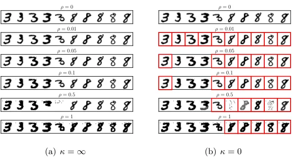
d((x1, y1),(x2, y2)) =kx1−x2k+κ|y1−y2| (11) for some κ >0.1 _{Note thatκ captures the costs of moving probability mass along the output} space. For κ = ∞ all distributions in the Wasserstein ball Bρ(Pb_N) are thus obtained by

reshaping Pb_N only along the input space. It is easy to verify that for κ=∞ and Ξ =Rn+1

the learning models portrayed in Corollaries 5-7 all simplify to

inf w 1 N N X i=1

L(hw,x_bii −ybi) +ckwk∗, (12)

where c=ρδ for robust regression with Huber loss, c=ρ for support vector regression with

-insensitive loss and c= max{τ,1−τ}ρ for quantile regression with pinball loss. Thus, (12) is easily identified as an instance of the classical regularized learning problem (2), where the dual norm term kwk∗ plays the role of the regularization function, while c represents

the usual regularization weight. By definition of the dual norm, the penalty kwk∗ assigned to a hypothesis w is maximal (minimal) if the cost of moving probability mass along w is minimal (maximal). We emphasize that if κ= ∞, then the marginal distribution of y

corresponding to every Q∈_Bρ(Pb_N) coincides with the empirical distribution _N1

PN

i=1δbyi.

Thus, classical regularization methods, which correspond to κ = ∞, are explained by a counterintuitive probabilistic model, which pretends that any training sample must have an output that has already been recordeded in the training dataset. In other words, classical regularization implicitly assumes that there is no uncertainty in the outputs. More intuitively appealing regularization schemes are obtained for finite values of κ.

To establish a connection between distributionally robust and classical robust regression as discussed in (El Ghaoui and Lebret, 1997; Xu et al., 2010), we further investigate the worst-case expected loss of a fixed linear hypothesis w.

sup Q∈Bρ(PbN)

EQ[L(hw,xi −y)] (13)

Theorem 9 (Extremal distributions in linear regression) The following statements hold.

(i) If L(z) = maxj≤J{ajz+bj}, then the worst-case expectation (13) coincides with



              

              

sup αij,qij,vij

1

N

N

X

i=1 J

X

j=1

αij aj(hw,xbii −ybi) +bj

+aj(hw,qiji −vij)

s.t. 1 N

N

X

i=1 J

X

j=1

k(qij, vij)k ≤ρ

J

X

j=1

αij = 1 i∈[N]

(xib +qij/αij,ybi+vij/αij)∈Ξ i∈[N], j∈[J]

αij ≥0 i∈[N], j∈[J]

(14)

for any fixed hypothesisw. Moreover, if(α?

ij,q?ij, v?ij)maximizes (14), then the discrete distribution

Q∗ = 1

N

N

X

i=1 J

X

j=1

α?_ijδ(xbi+q ?

ij/α?ij,ybi+v ? ij/α?ij),

represents a maximizer for (13).

(ii) If Ξ =Rn+1 and L(z) is Lipschitz continuous, then the discrete distributions

Qγ= 1

N

N

X

i=2

δ(xbi,ybi)+

1−γ

N δ(x1b ,by1)+

γ Nδ(x1b +

ρN γ x?,yb1+

ρN

γ y?)

for γ ∈(0,1],

where (x?_{, y}?_{) solves max}

Recall that 0/0 = 0 and 1/0 =∞ by our conventions of extended arithmetic. Thus, any solution feasible in (14) with αij = 0 must satisfyqij =0 and vij = 0 because otherwise (xbi+qij/αij,ybi+vij/αij)∈/ Ξ.

Theorem 9 shows how one can use convex optimization to construct a sequence of distributions that are asymptotically optimal in (13). Next, we argue that the worst-case expected cost (13) is equivalent to a (robust) worst-worst-case cost over a suitably defined uncertainty set if the following assumption holds.

Assumption 10 (Minimal dispersion) For every w ∈ _Rn _{there is a training sample} (x_bk,ybk) for some k ≤ N such that the derivative L

0 _{exists at hw,}

b

xki −ybk and satisfies

|L0(hw,xkb i −byk)|= lip(L).

Remark 11 (Minimal dispersion) Assumption 10 is reminiscent of the non-separability condition in (Xu et al., 2009, Theorem 3), which is necessary to prove the equivalence of robust and regularized support vector machines. In the regression context studied here, Assumption 10 ensures that, for every w, there exists a training sample that activates the largest absolute slope of L.

For instance, in support vector regression, it means that for every w there exists a data point outside of the slab of width 2/k(w,−1)k2 centered around the hyperplane Hw=

{(x, y)∈_Rn_×

R:hw,xi−y= 0}(i.e., the empirical-insensitive loss is not zero). Similarly, in robust regression with the Huber loss function, Assumption 10 stipulates that for every w there exists a data point outside of the slab of width 2δ/k(w,−1)k2 centered around Hw.

However, quantile regression with τ 6= 0.5 fails to satisfy Assumption 10. Indeed, for any training dataset there always exists some w such that all data points reside on the side of

Hw where the pinball loss function is less steep.

Theorem 12 (Robust regression) If Ξ =Rn+1 and the loss function L(z) is Lipschitz continuous, then the worst-case expected loss (13) provides an upper bound on the (robust) worst-case loss



    

    

sup ∆xi,∆yi

1

N

N

X

i=1

[L(hw,xib + ∆xii −ybi−∆yi)]

s.t. 1 N

N

X

i=1

k(∆xi,∆yi)k ≤ρ.

(15)

Moreover, if Assumption 10 holds, then (13) and (15) are equal.

Remark 13 (Tractability of robust regression) Assume that Ξ =Rn+1, while L and

3.2. Distributionally Robust Linear Classification

Throughout this section we focus on linear classification problems, where `(hw,xi, y) =

L(yhw,xi) for some convex univariate loss functionL. We also assume thatXis both convex and closed and that Y={+1,−1}. Moreover, we assume that the transportation metricd is defined via

d((x, y),(x0, y0)) =kx−x0k+κ1{y6=y0_}, (16)

wherek·krepresents a norm on the input spaceRn, andκ >0 quantifies the cost of switching a label. In this setting, the distributionally robust classification problem (4) admits an equivalent reformulation as a finite convex optimization problem if either (i) the univariate loss function L is piecewise affine or (ii) X= Rn and L is Lipschitz continuous (but not necessarily piecewise affine).

Theorem 14 (Distributionally robust linear classification) The following statements hold.

(i) If L(z) = maxj∈J{ajz+bj}, then (4)is equivalent to



       

       

inf

w,λ,si

p+_ij,p−_ij

λρ+ 1

N

N

X

i=1

si

s.t. S_X(ajybiw−p

+

ij) +bj +hp+ij,xbii ≤si i∈[N], j∈[J]

S_X(−ajbyiw−p

−

ij) +bj+hp −

ij,xib i −κλ≤si i∈[N], j∈[J]

kp+_ijk∗ ≤λ,kp−_ijk∗ ≤λ i∈[N], j∈[J],

(17)

where S_X denotes the support function of X.

(ii) If X=Rn and L is Lipschitz continuous, then (4) is equivalent to



     

     

inf

w,λ,si

λρ+ 1

N

N

X

i=1

si

s.t. L(_byihw,xbii)≤si i∈[N]

L(−y_bihw,xibi)−κλ≤si i∈[N]

lip(L)kwk∗≤λ.

(18)

In the following, we exemplify Theorem 14 for the hinge loss, logloss and smoothed hinge loss functions under the assumption that the input spaceXadmits the conic representation

X={x∈Rn:CxC d} (19)

Corollary 15 (Support vector machine) If L represents the hinge loss function and X is of the form (19), then (4) is equivalent to

                     inf w,λ si,p+i,p

−

i

λρ+ 1

N

N

X

i=1

si

s.t. 1−y_bi(hw,xibi) +hp

+

i ,d−Cxibi ≤si i∈[N]

1 +ybi(hw,xbii) +hp

−

i ,d−Cxbii −κλ≤si i∈[N]

kC>p+_i +y_biwk∗ ≤λ, kC>p−_i −byiwk∗ ≤λ i∈[N]

si≥0, p+_i ,p−_i ∈ C∗ i∈[N].

(20)

Corollary 16 (Support vector machine with smooth hinge loss) IfLrepresents the smooth hinge loss function and X=Rn, then (4)is equivalent to

                       min

w,λ,si

z+_i,z−_i ,t+_i,t−_i

λρ+ 1

N

N

X

i=1

si

s.t. 1₂(z_i+−y_bihw,xibi)

2_+t+

i ≤si i∈[N] 1

2(z −

i +ybihw,xbii)

2_+t−

i −κλ≤si i∈[N] 1−z_i+≤t+_i , 1−z_i−≤t−_i i∈[N]

t+_i , t−_i ≥0 i∈[N]

kwk∗≤λ.

(21)

Corollary 17 (Logistic regression) If L represents the logloss function and X = Rn, then (4) is equivalent to

                   min

w,λ,si

λρ+ 1

N

N

X

i=1

si

s.t. log1 + exp −y_bihw,xib i

≤si i∈[N]

log1 + exp y_bihw,xib i

−κλ≤si i∈[N]

kwk∗ ≤λ.

(22)

Remark 18 (Relation to classical regularization) If X=Rn and the weight parame-ter κin the transportation metric (16)is set to infinity, then the learning problems portrayed in Corollaries 15–17 all simplify to

inf w 1 N N X i=1

L(y_bihw,xbii) +ρkwk∗. (23)

X, but it cannot flip outputs from +1 to −1 or vice versa. Thus, classical regularization schemes, which are recovered for κ=∞, implicitly assume that output measurements are exact. As this belief is not tenable in most applications, an approach with κ <∞ may be more satisfying. We remark that alternative approaches for learning with noisy labels have previously been studied by Lawrence and Sch¨olkopf (2001), Natarajan et al. (2013), and Yang et al. (2012).

Remark 19 (Relation to Tikhonov regularization) The learning problem

inf w 1 N N X i=1

L(ybihw,xib i) +ckwk

2

2 (24)

with Tikhonov regularizer enjoys wide popularity. IfL represents the hinge loss, for example, then (24)reduces to the celebrated soft margin support vector machine problem. However, the Tikhonov regularizer appearing in (24) is not explained by a distributionally robust learning problem of the form (4). It is known, however, that (23) with k · k∗ =k · k2 and (24) are equivalent in the sense that for every ρ≥0 there exists c≥0 such that the solution of (23) also solves (24) and vice versa (Xu et al., 2009, Corollary 6).

To establish a connection between distributionally robust and classical robust classification as discussed in (Xu et al., 2009), we further investigate the worst-case expected loss of a fixed linear hypothesis w.

sup Q∈Bρ(Pb_N)

EQ[L(yhw,xi)] (25)

Theorem 20 (Extremal distributions in linear classification) The following state-ments hold.

(i) If L(z) = maxj∈J{ajz+bj}, then the worst-case expectation (25) coincides with

                                     sup α+_ij,α−_ij

q+_ij,q−_ij

1 N N X i=1 J X j=1

(α+_ij −α−_ij)ajybihw,xib i+ajybihw,q

+ ij −q

− iji+

J

X

j=1

bj

s.t.

N X i=1 J X j=1

kq+_ijk+kq_ij−k+κα−_ij ≤N ρ

J

X

j=1

α+_ij+α−_ij = 1 i∈[N]

b

xi+q+ij/αij+∈X, xbi+q

− ij/α

−

ij ∈X i∈[N], j ∈[J]

α+_ij, α−_ij ≥0 i∈[N], j ∈[J]

(26)

for any fixed w. Also, if (α+_ij?, α−_ij?,q+_ij?,q_ij−?) maximizes (26), then the discrete distribution

Q= 1

N N X i=1 J X j=1

α+_ij?δ₍

b

xi−q+ij ?

/α+_ij?,ybi)

+α−_ij?δ₍

b

xi−q−ij ?

/α−_ij?,−ybi)

(ii) If X=Rn, then the worst-case expectation (25) coincides with the optimal value of



        

        

sup αi,θ

lip(L)k(w)k∗θ+ 1

N

N

X

i=1

(1−αi)L(ybihw,xbii) +αiL(−ybihw,bxii)

s.t. θ+ κ

N

N

X

i=1

αi =ρ−γ

0≤αi ≤1 i∈[N]

θ≥0

(27)

for γ = 0. Moreover, if (α?

i(γ), θ?(γ)) maximizes (27) for γ > 0, η(γ) =γ/(θ?(γ) +

κ−ρ+γ+ 1) andx? solves maxx{hw,xi:kxk ≤1}, then the discrete distributions

Qγ = 1

N

N

X

i=2

(1−α?_i(γ))δ(xbi,byi)+α

?

i(γ)δ(xbi,−ybi)+

η(γ)

N δ(x1b + θ?(γ)N

η(γ) x

?_, b

y1)

+1−η(γ)

N

h

(1−α?₁(γ))δ₍

b

x1,by1)+α

?

1(γ)δ(x1b ,−yb1) i

for γ ∈[0,min{ρ,1}]are feasible and asymptotically optimal in (25) for γ ↓0. Theorem 20 shows how one can use convex optimization to construct a sequence of distributions that are asymptotically optimal in (25). Next, we show that the worst-case expected cost (25) is equivalent to a (robust) worst-worst-case cost over a suitably defined uncertainty set if the following assumption holds.

Assumption 21 (Non-separability) For everyw∈Rnthere is a training sample(xbk,ybk)

for somek≤N such that the derivativeL0 exists atybkhw,xbkiand satisfies|L

0₍

b

ykhw,xbki)|=

lip(L).

Remark 22 (Non-separability) Assumption 21 generalizes the non-separability condition in (Xu et al., 2009, Theorem 3) for the classical and smooth hinge loss functions to more general Lipschitz continuous losses. Note that, in the case of the hinge loss, Assumption 21 effectively stipulates that for anywthere exists a training sample(xbk,ybk)withybkhw,xbki<1,

implying that the dataset cannot be perfectly separated by any linear hypothesis w. An equivalent requirement is that the empirical hinge loss is nonzero for every w. Similarly, in the case of the smooth hinge loss, Assumption 21 ensures that for any w there is a training sample with _bykhw,xbki <0, which implies again that the dataset admits no perfect linear

separation. Note, however, that the logloss fails to satisfy Assumption 21 as its steepest slope is attained at infinity.

Theorem 23 (Robust classification) Suppose that X=Rn, the loss functionL is Lips-chitz continuous and the cost of flipping a label in the transportation metric (16) is set to

κ =∞. Then, the worst-case expected loss (25) provides an upper bound on the (robust) worst-case loss



    

    

sup ∆xi

1

N

N

X

i=1

L(y_bihw,xbi+ ∆xii)

s.t. 1 N

N

X

i=1

k∆xik ≤ρ.

Moreover, if Assumption 21 holds, then (25) and (28) are equal.

Remark 24 (Tractability of robust classification) Assume thatX=Rn, while L and

k · k both admit a tractable conic representation. By Theorem 14, the worst-case expected loss (25) can then be computed in polynomial time by solving a tractable convex program. Theorem 23 thus implies that the worst-case loss (28) can also be computed in polynomial time if Assumption 21 holds. This confirms Proposition 4 in (Xu et al., 2009). No efficient method for computing (28) is know if Assumption 21 fails to hold.

3.3. Nonlinear Hypotheses: Reproducing Kernel Hilbert Spaces

We now generalize the learning models from Sections 3.1 and 3.2 to nonlinear hypotheses that range over areproducing kernel Hilbert space(RKHS)H⊆RXwith inner producth·,·iH.

By definition,H thus constitutes a complete metric space with respect to the normk · kH

induced by the inner product, and the point evaluationh 7→h(x) of the functionsh∈H represents a continuous linear functional onHfor any fixedx∈X. The Riesz representation theorem then implies that for everyx∈_Xthere exists a unique function Φ(x)∈_Hsuch that

h(x) =hh,Φ(x)i_H for all h∈H. We henceforth refer to Φ :X→Has thefeature map and tok:X×X→R+ withk(x,x0) =hΦ(x),Φ(x0)iH as thekernel function. By construction,

the kernel function is symmetric and positive definite, that is, thekernel matrix K∈_RN×N defined throughKij =k(xi,xj) is positive definite for all N ∈Nand {xi}i≤N ⊆X.

By the Moore-Aronszajn theorem, any symmetric and positive definite kernel function k

on Xinduces a unique RKHS H⊆RX, which can be represented as

H=

(

h∈_RX_:∃β

i ∈R, xi∈X∀i∈Nwithh(x) = ∞

X

i=1

βik(xi,x) and

∞

X

i=1 ∞

X

j=1

βik(xi,xj)βj <∞

)

,

where the inner product of two arbitrary functions h1, h2 ∈Hwithh1(x) =P∞_i=1βik(xi,x) andh2(x) =

P∞

j=1β 0 jk(x

0

j,x) is defined as hh1, h2iH=

P∞

i=1

P∞

j=1βik(xi,x0j)β 0

j. One may now use the kernel function to define the feature map Φ through [Φ(x0_{)](x) = k(x}0_,x) for all x,x0 ∈X. This choice is admissible because it respects the consistency condition

hΦ(x),Φ(x0)i_H=k(x,x0) for all x,x0∈_H, and because it implies the desiredreproducing property hf,Φ(x0_)i

H =

P∞

i=1βik(xi,x0) =f(x0) for all f ∈Hand x0 ∈X.

In summary, given a symmetric and positive definite kernel function k, there exists an associated RKHS Hand a feature map Φ with the reproducing property. As we will see below, however, to optimize over nonlinear hypotheses in H, knowledge of k is sufficient, and there is no need to constructHand Φ explicitly.

Assume now that we are given any symmetric and positive definite kernel function k, and construct a distributionally robust learning problem over all nonlinearhypotheses in the corresponding RKHS Hvia

b

J(ρ) = inf h∈H

sup Q∈Bρ(PbN)

where the transportation metric is given by the Euclidean norm on X×Y(for regression problems) or the separable metric (16) with the Euclidean norm on X (for classification problems). While problem (29) is hard to solve in general due to the nonlinearity of the hypothesesh∈_H, it is easy to solve a lifted learning problem where the inputs x∈_Xare replaced with featuresx_H∈H, while eachnonlinearhypothesish∈Hover the input space Xis identified with alinearhypothesishH ∈Hover the feature spaceHthrough the identity h_H(x_H) =hh,x_Hi_H. Thus, the lifted learning problem can be represented as

b

J_H(ρ) = inf h∈H

sup Q∈Bρ(PbH_N)

EQ[`(hh,x_Hi_H, y)], (30)

wherePbH_N = 1/N

PN

i=1δ(Φ(xbi),ybi) onH×Ydenotes the pushforward measure of the emprical

distribution Pb_N under the feature map Φ induced by k, while Bρ(PbH_N) constitutes the

Wasserstein ball of radiusρ around PbH_N corresponding to the transportation metric

d_H (x_H, y),(x0_H, y0)

=

( q

kx_H−x0

Hk

2

H+ (y−y

0₎2 _{for regression problems,}

kx_H−x0

HkH+κ1{y6=y0_} for classification problems.

Even thoughPbH_N constitutes the pushforward measure ofPb_N under Φ, not every distribution

QH _{∈ B}

ρ(PbH_N) can be obtained as the pushforward measure of some Q∈ B_ρ(Pb_N). Thus,

we should not expect (29) to be equivalent to (30). Instead, one can show that under a judicious transformation of the Wasserstein radius, (30) provides an upper bound on (29) whenever the kernel function satisfies a calmness condition.

Assumption 25 (Calmness of the kernel) The kernel function k is calm from above, that is, there exist a concave smooth growth function g : R+ → R+ with g(0) = 0 and

g0(z)≥1 for all z∈R+ such that

p

k(x1,x1)−2k(x1,x2) +k(x2,x2)≤g(kx1−x2k2) ∀x1,x2∈X.

The calmness condition is non-restrictive. In fact, it is satisfied by most commonly used kernels.

Example 1 (Growth Functions for Popular Kernels) For most commonly used ker-nelskonX⊆Rn, we can construct an explicit growth functiong that certifies the calmness of

k in the sense of Assumption 25. This construction typically relies on elementary estimates. Derivations are omitted for brevity.

1. Linear kernel: For k(x1,x2) =hx1,x2i, we may set g(z) =z.

2. Gaussian kernel: For k(x1,x2) = e−γkx1−x2k

2

2 with γ > 0, we may set g(z) =

max{√2γ,1}z.

3. Laplacian kernel: For k(x1,x2) = e−γkx1−x2k1 _{with γ > 0, we may set g(z) =}

p

4. Polynomial kernel: The kernelk(x1,x2) = (γhx1,x2i+ 1)d with γ >0 and d∈N fails to satisfy the calmness condition if X is unbounded and d > 1, in which case

p

k(x1,x1)−2k(x1,x2) +k(x2,x2) grows superlinearly. IfX⊆ {x∈Rn:kxk2 ≤R} for some R > 0, however, the polynomial kernel is calm with respect to the growth function

g(z) =

(

max{ 1 2R

p

2(γR2_{+ 1)}d_{,1}z if dis even,} max{_2R1 p2(γR2_{+ 1)}d_−2(1−γR2₎d_{,1}z if dis odd.}

Theorem 26 (Lifted learning problems) If Assumption 25 holds for some growth func-tion g, then the following statements hold for all Wasserstein radii ρ≥0.

(i) For regression problems we have Jb(ρ)≤Jb_H(

√

2g(ρ)).

(ii) For classification problems we have Jb(ρ)≤Jb_H(g(ρ)).

We now argue that the lifted learning problem (30) can be solved efficiently by lever-aging the following representer theorem, which generalizes (Sch¨olkopf and Smola, 2001, Theorem 4.2) to non-separable loss functions.

Theorem 27 (Representer theorem) Assume that we are given a symmetric positive definite kernelkonXwith corresponding RKHS H, a set of training samples (xib ,ybi)∈X×Y,

i≤N, and an arbitrary loss function f : (X×Y×R)N×R+→R that is non-decreasing in its last argument. Then, there exist βi ∈R, i≤N, such that the learning problem

min

h∈_H f((x1b ,by1, h(x1))b , . . . ,(xNb ,ybN, h(xNb )),khkH) (31)

is solved by a hypothesis h? _∈

H representable ash?(x) =PNi=1βik(x,xi).b

The subsequent results involve the Kernel matrix K = [Kij] defined through Kij =

k(xbi,xbj),i, j≤N. The following theorems demonstrate that the lifted learning problem (30)

admits a kernel representation.

Theorem 28 (Kernelized distributionally robust regression) Suppose thatX=Rn, Y = R and k is a symmetric positive definite kernel on X with associated RKHS H. If

` is generated by a convex and Lipschitz continuous loss function L, that is, `(h(x), y) =

L(h(x)−y), then (30) is equivalent to

min

β∈_RN

1

N

N

X

i=1

L

N

X

j=1

Kijβj −ybi

+ρlip(L)k(K12β,1)k₂,

and for any of its minimizersβ? the hypothesis h?_{(x) =}PN

i=1βi?k(x,xi)b is optimal in (30).

RKHS H. If `is generated by a convex and Lipschitz continuous loss function L, that is,

`(h(x), y) =L(yh(x)), then (30) is equivalent to



            

            

min βi,λ,si

λρ+ 1

N

N

X

i=1

si

s.t. L

N

X

j=1

b

yiKijβj

≤si i∈[N]

L−

N

X

j=1

b

yiKijβj

−κλ≤si i∈[N]

lip(L)kK12βk₂ ≤λ,

(32)

and for any of its minimizersβ? the hypothesis h?_{(x) =}PN

i=1βi?k(x,xbi) is optimal in (30).

Theorems 28 and 29 show that the lifted learning problem (30) can be solved with similar computational effort as problem (4), that is, optimizing over a possibly infinite-dimensional RKHS of nonlinear hypotheses is not substantially harder than optimizing over the space of linear hypotheses.

Remark 30 (Kernelization in robust regression and classification) Recall from The-orem 12 that distributionally robust and classical robust linear regression are equivalent if Ξ =Rn+1 and the training samples are sufficiently dispersed in the sense of Assumption 10. Similarly, Theorem 23 implies that distributionally robust and classical robust linear classifi-cation are equivalent ifκ=∞ and the training samples are non-separable in the sense of Assumption 21. One can show that Theorems 12 and 23 naturally extend to nonlinear regres-sion and classification models over an RKHS induced by some symmetric and positive definite kernel. Specifically, one can show that some lifted robust learning problem is equivalent to the lifted distributionally robust learning problem (30) whenever the lifted training samples (Φ(x1)b ,by1),· · · ,(Φ(xbN),ybN)satisfy Assumption 10 (for regression) or 21 (for classification).

Theorems 28 and 29 thus imply that the lifted robust regression and classification problems can be solved efficiently under mild regularity conditions whenever Assumptions 10 and 21 hold, respectively. Unfortunately, these conditions are often violated for popular kernels. For example, the lifted samples are always linearly separable under the Gaussian kernel (Xu et al., 2009, p. 1496). In this case, the lifted robust classification problem can never be reduced to an efficiently solvable lifted distributionally robust classification problem of the form (30). In fact, no efficient method for solving the lifted robust classification problem seems to be known. In contrast, the lifted distributionally robust learning problems are always efficiently solvable under standard regularity conditions.

3.4. Nonlinear Hypotheses: Neural Networks2

Families ofneural networksrepresent particularly expressive classes of nonlinear hypotheses. In the following, we characterize a familyHof neural networks with M ∈Nlayers through

M continuous activation functions σm : Rnm+1 → Rnm+1 and M weight matrices Wm ∈

Rnm+1×nm,m∈[M]. The weight matrices can encodefully connectedorconvolutionallayers, for example. If n1=nand nM+1 = 1, then we may set

H=

n

h∈_RX_{:∃Wm ∈}

Rnm+1×nm, m∈[M], h(x) =σM

WM· · ·σ2 W2σ1(W1x)

· · ·o.

Each hypothesis h ∈ _H constitutes a neural network and is uniquely determined by the collection of all weight matrices W[M] := (W1, . . . ,WM). In order to emphasize the dependence on W[M], we will sometimes use h(x;W[M]) to denote the hypotheses in H. Settingx1 =x, the features of the neural network are defined recursively throughxm+1=

σm(zm), wherezm=Wmxm, m∈[M]. The features xm, m= 2, . . . , M, correspond to the hiddenlayers of the neural network, while xM+1 determines its output.

Example 2 (Activation functions) The following activation functions are most widely used.

1. Hyperbolic tangent: [σm(zm)]i= (exp(2[zm]i)−1)/(exp(2[zm]i) + 1)

2. Sigmoid: [σm(zm)]i = 1/(1 + exp(−[zm]i))

3. Softmax: [σm(zm)]i = exp([zm]i)/Pnj=1m+1exp([zm]j)

4. Rectified linear unit (ReLU): [σm(zm)]i = max{0,[zm]i}

5. Exponential linear unit (ELU):[σm(zm)]i = max{0,[zm]i}+min{0, α(exp([zm]i)−

1)}

The distributionally robust learning model over the hypothesis class H can now be represented as

inf

h∈_H sup Q∈Bρ(Pb_N)

EQ` h(x), y

= inf

W[M]

sup Q∈Bρ(Pb_N)

EQ` h(x;W[M]), y

, (33)

where we use the transportation metrics (11) and (16) for regression and classification problems, respectively. Moreover, we adopt the standard convention that `(h(x), y) =

L(h(x)−y) for regression problems and `(h(x, y)) =L(yh(x)) for classification problems, where Lis a convex and Lipschitz continuous univariate loss function. In the following we equip each feature space Rnm with a normk · k,m∈[M + 1]. By slight abuse of notation, we use the same symbol for all norms even though the norms on different feature spaces may differ. Using the norm on Rnm+1, we define the Lipschitz modulus ofσm as

lip(σm) := sup

z,z0_∈ Rnm+1

kσ(z)−σ(z0)k

kz−z0k :z 6=z

0

.

Theorem 31 (Distributionally robust learning with neural networks) The distri-butionally robust learning model (33) is bounded above by the regularized empirical loss minimization problem

inf

W[M]

1

N

N

X

i=1

`(h(xi;b W[M]),ybi) +ρlip(L) max

( _M

Y

m=1

lip(σm)kWmk,c κ

)

, (34)

where c= 1 for regression problems andc= max{1,2 sup_h∈_H,x∈_X|h(x)|} for classification problems. Moreover, kWmk = supkxmk=1kWmxmk is the operator norm induced by the

norms on Rnm and Rnm+1.

Remark 32 (Uniform upper bound on all neural networks) For classification prob-lems the constant c in (34) represents a uniform upper bound on all neural networks and may be difficult to evaluate in general. It is easy to estimatec, however, if the last activation function is itself bounded such as the softmax function, which yields a probability distribution over the output space. In this case one may simply set c= 2.

The product termQM

m=1lip(σm)kWmkin (34) represents an upper bound on the Lipschitz modulus of h(x;W_[M]). We emphasize that computing the exact Lipschitz modulus of a neural network is NP-hard even if there are only two layers and all activation functions are of the ReLU type (Scaman and Virmaux, 2018, Theorem 2). In contrast, the upper bound at hand is easy to compute as all activation functions listed in Example 2 have Lipschitz modulus 1 with respect to the Euclidean norms on the domain and range spaces (Gouk et al., 2018; Wiatowski et al., 2016). For more details on how to estimate the Lipschitz moduli of neural networks we refer to (Gouk et al., 2018; Miyato et al., 2018; Neyshabur et al., 2018; Szegedy et al., 2013).

Note that even though (34) represents a finite-dimensional optimization problem over the weight matrices of the neural network, both the empirical prediction loss as well as the regularization term are non-convex inW[M], which complicates numerical solution. If

κ=∞, however, one can derive an alternative upper bound on the distributionally robust learning model (33) with a convexregularization term.

Corollary 33 (Convex regularization term) If κ =∞, then there is ρ ≥0 such that the distributionally robust learning model (33) is bounded above by the regularized empirical loss minimization problem

inf

W[M]

1

N

N

X

i=1

`(h(xi;b W[M]),ybi) +ρ

M

X

m=1

kWmk. (35)

As the empirical prediction loss remains non-convex, it is expedient to address prob-lem (35) with local optimization methods such as stochastic gradient descent algorithms. For a comprehensive review of first- and the second-order stochastic gradient algorithms we refer to (Agarwal et al., 2017) and the references therein. In the numerical experiments we will use a stochastic proximal gradient descent algorithm that exploits the convexity of the regularization term and generates iterates W_[Mk _] fork∈Naccording to the update rule

W_mk+1 = prox_ηkρkWmk

W_mk −ηk∇Wm`(h(xibk;W

k

[M]),ybik)

where ηk > 0 is a given step size and ik is drawn randomly from the index set [N], see, e.g., Nitanda (2014). Here, the proximal operator associated with a convex function

ϕ:Rnm+1×nm →Ris defined through

prox_ϕ(Wm) := arg min

W0

m

ϕ(W_m0 ) +1 2kW

0

m−Wmk2F,

where k · k_F stands for the Frobenius norm. The algorithm is stopped as soon as the improvement of the objective value falls below a prescribed threshold. As the empirical prediction loss is non-convex and potentially non-smooth, the algorithm fails to offer any strong performance guarantees. For the scalability of the algorithm, however, it is essential that the proximal operator can be evaluated efficiently.

Example 3 (Proximal operator) Suppose that all feature spacesRnm are equipped with the p-norm for some p ∈ {1,2,∞}, which implies that all parameter spaces Rnm+1×nm are equipped with the corresponding matrix p-norm. In this case the proximal operator of

ϕ(Wm) =ηkWmkp for some fixed η >0 can be evaluated highly efficiently.

1. MACS (p = 1): The matrix 1-norm returns the maximum absolute column sum

(MACS). Evaluating the proximal operator ofϕ(Wm) =ηkWmk1 amounts to solving the minimization problem

prox_ϕ(Wm) =



 

 

min

W0

m,u

ηu+ nm X

i=1

k[W_m0 ]:,i−[Wm]:,ik2₂

s.t. k[W0

m]:,ik1 ≤u i∈[nm],

where[Wm]:,iand[Wm0 ]:,irepresent thei-th columns of Wm and Wm0 , respectively. For any fixed u, the above problem decomposes into nm projections of the vectors [Wm]:,i,

i∈[nm], to the `1-ball of radius u centered at the origin. Each of these projections can be computed via an efficient sorting algorithm proposed in (Duchi et al., 2008). Next, we can use any line search method such as the golden-section search algorithm to optimize overu, thereby solving the full proximal problem.

2. Spectral (p= 2): The matrix 2-norm coincides with the spectral norm, which returns

the maximum singular value. In this case, the proximal problem forϕ(Wm) =ηkWmk2 can be solved analytically via singular value thresholding (Cai et al., 2010, Theorem 2.1), that is, given the singular value decomposition Wm =U SV> with U ∈Rnm+1×nm+1 orthogonal, S ∈ _Rnm+1×nm

+ diagonal and V ∈ Rnm×nm orthogonal, the proximal operator satisfies

prox_ϕ(Wm) = prox_ϕ(U SV>) =USVe >, where Sije = max{Sij−η,0}.

The singular value decomposition can be accelerated using a randomized algorithm proposed in (Halko et al., 2011).

3. MARS (p = ∞): The matrix ∞-norm returns the maximum absolute row sum

The convergence behavior of the stochastic proximal gradient descent algorithm can be further improved by including a momentum term inside the proximal operator, see, e.g., Loizou and Richt´arik (2017).

4. Generalization Bounds

Generalization bounds constitute upper confidence bounds on the out-of-sample error. Tra-ditionally, generalization bounds are derived by controlling the complexity of the hypothesis space, which is typically quantified in terms of its VC-dimension or via covering numbers or Rademacher averages (Shalev-Shwartz and Ben-David, 2014). Strengthened generaliza-tion bounds for large margin classifiers can be obtained by improving the estimates of the VC-dimension and the Rademacher average (Shivaswamy and Jebara, 2007, 2010). We will now demonstrate that distributionally robust learning models of the type (4) or (30) enjoy simple new generalization bounds that can be obtained under minimal assumptions. In particular, they do not rely on any notions of hypothesis complexity and may therefore even extend to hypothesis spaces with infinite VC-dimensions. Our approach is reminiscent of the generalization theory for robust support vector machines portrayed in (Xu et al., 2009), which also replaces measures of hypothesis complexity with robustness properties. However, we derive explicit finite sample guarantees, while (Xu et al., 2009) establishes asymptotic consistency results. Moreover, we relax some technical conditions used in (Xu et al., 2009) such as the compactness of the input spaceX.

The key enabling mechanism of our analysis is a measure concentration property of the Wasserstein metric, which holds whenever the unknown data-generating distribution has exponentially decaying tails.

Assumption 34 (Light-tailed distribution) There exist constants a > 1 and A > 0 and a reference point ξ0 ∈ Rn+1 such that EP[exp (d(ξ,ξ0))a)] ≤ A, where d denotes the usual mass transportation cost.

Theorem 35 (Measure concentration (Fournier and Guillin, 2015, Theorem 2)) If Assumption 34 holds, then we have

PNnW(P,Pb_N)≥ρ o

≤

c1exp −c2N ρmax{n+1,2}

if ρ≤1, c1exp −c2N ρa

if ρ >1, (36)

for all N ≥1, n6= 1, andρ >0, where the constants c1, c2 >0 depend only on a, A,d and

n.3

Theorem 35 asserts that the empirical distribution Pb_N converges exponentially fast to

the unknown data-generating distributionP, in probability with respect to the Wasserstein metric, as the sample size N tends to infinity. We can now derive simple generalization bounds by increasing the Wasserstein radiusρ until the violation probability on the of the right hand side of (36) drops below a prescribed significance level η ∈(0,1]. Specifically,