Model Selection via the VC Dimension

Model Selection via the VC Dimension

Merlin Mpoudeu [email protected]

Bank of America Atlanta, GA, USA

Bertrand Clarke [email protected]

Department of Statistics University of Nebraska-Lincoln Lincoln, NE 68503, USA

Editor:John Shawe-Taylor

Abstract

We derive an objective function that can be optimized to give an estimator for the Vapnik-Chervonenkis dimension for use in model selection in regression problems. We verify our estimator is consistent. Then, we verify it performs well compared to seven other model selection techniques. We do this for a variety of types of data sets.

Keywords: Vapnik-Chervonenkis dimension, model selection, Bayesian information cri-terion, sparsity methods, empirical risk minimization, multi-type data.

1. Complexity and Model Selection

Model selection is often the first problem that must be addressed when analyzing data. In M-closed problems, see Bernardo and Smith (2000), the analyst posits a list of models and assumes one of them is true. In such cases, model selection is any procedure that uses data to identify one of the models on the model list. There is a vast literature on model selection in this context including information based methods such as the Aikaikie Information Criterion (AIC), the Bayes information criterion (BIC), residual based methods such as MallowsCp or branch and bound, and code length methods such as the two-stage coding proposed by Barron and Cover (1991). We also have computational search methods such as simulated annealing and genetic algorithms. In addition, cross-validation (CV) is often used with non-parametric methods such as recursive partitioning, neural networks (aka deep learning) and kernel methods. A less well developed approach to model selection is via complexity as assessed by the Vapnik-Chervonenkis (VC) dimension, here denoted by

dV C. Its earliest usage seems to be in Vapnik and Chervonenkis (1968). A translation into English was published as Vapnik and Chervonenkis (1971).

Although, the VC dimension goes back to 1968, it wasn’t until Vapnik et al. (1994) that a method for estimatingdV C was proposed in the classification context. Specifically, given a collection C of classifiers, Vapnik et al. (1994) tried to estimate the VC dimension of C by deriving an objective function based on the expected value of the maximum difference between two empirical evaluations of a single loss function, here denoted by ∆. The two empirical values come from dividing a given data set into a first and second part. The

c

objective function proposed by Vapnik et al. (1994) depends ondV C, the sample sizen, and several constants that had to be determined. Using their objective function, they derived an estimator ˆdV C fordV C given a classCof classifiers. This algorithm treated possible sample sizes as design points n1, n2,· · · , nL and requires one level of bootstrapping. Despite the remarkable contribution of Vapnik et al. (1994), the objective function was over-complex and the algorithm did not give a tight enough bound on ∆. Later, Vapnik and his collaborators suggested a fix to tighten the bound on ∆. We do not use this here; it is unclear if this ‘fix’ will work in classification, let alone regression.

Choosing the design points is a nontrivial source of variability in the estimate of dV C. So, Shao et al. (2000) proposed an algorithm, based on extensive simulations, to generate optimal values ofn1, n2,· · ·, nL, givenL. They argued that non-uniform values of thenl’s gave better results than the uniformnl’s used in Vapnik et al. (1994).

More recently, in a pioneering paper that deserves more recognition that it has received, McDonald et al. (2011) established the consistency of the Vapnik (1998) estimator ˆdV C for

dV C in the classification context.

The main reason the estimator for dV C of Vapnik et al. (1994) did not become more widely used, despite the result in McDonald et al. (2011), is, we suggest, that it was too unstable because the objective function did not bound ∆ tightly enough in terms ofdV C. In addition, the form of the objective function in Vapnik et al. (1994) is more complicated and less well-motivated than our result Theorem 2. The reason is that the derivation in Vapnik et al. (1994) uses conditional probabilities, one of which goes to zero quite quickly (withn). So, it contributes negligibly to the upper bound. Our derivation ignores the conditioning and bounds a CV form of ∆ that is typically larger than that used in Vapnik et al. (1994).

Our consistency proof is a simplification of the proof of the main result McDonald et al. (2011). Accordingly, we obtain a slower rate of consistency, but the probability of correct model selection still goes to one.

when properly done, is fully competitive with existing methods and, unlike them, rarely gives abberant results.

This manuscript is structured as follows. In Sec. 2 we present the main theory justifying our estimator. In Subsec. 2.1 we discretize bounded loss functions so that upper bounds for the distinct regions involved in the definition of ∆ can be derived and in Subsec. 2.2 we define our estimator of the VC dimension and give an algorithm for how to compute it. In Sec. 3 we use McDonald et al. (2011)’s consistency theorem to motivate our consistency theorem for ˆdV C. In Sec. 4 we present our studies using simulated, benchmark, and real data. We compare our method for model selection to AIC, BIC, CV, P ERM\ 1, and

\

P ERM2. In this context, we suggest criteria to guide the selection of design points. Our comparisons also include simplifying non-nested model lists by using correlation, SCAD, and ALASSO. In Sec. 5 we discuss our overall findings.

2. Deriving an optimality criterion for estimating VC dimension

This section concerns ∆, the expected supremal difference between two evaluations of a bounded loss function, formally defined in (18) and (19). These bounds will enable us to derive an estimator for the VC dimension. In Sec. 2.1, we present our alternative version of the Vapnik et al. (1994) bounds and in Sec. 2.2, we present our estimator ofdV C.

2.1. Extension of the Vapnik et al. (1994) bounds to regression

Let Z = (X, Y) be a random variable with outcomes z = (x, y) assuming values on Z =

X × Y. The first entry,X=x, is regarded as an explanatory variable leading toY =y. Let

P ∈ M(Z) be the distribution ofZ, whereM(Z) is the collection of probability measures on

Z, and letZ1:2n= (Z1, . . . , Zn, Zn+1, . . . , . . . , Z2n) be a data set of size 2mof independently and identically distributed (IID) copies of Z. Write D1 = {Z₁, . . . , Zn} for the first half and D2={Zn+1, . . . , Z2n} for the second half. WritingZi= (Xi, Yi) for i= 1. . .2n, let

Q(Zi, α) =L(Yi, f(Xi, α)),

for a bounded real valued loss functionLandα∈Λ. We assume that Λ is a compact set in a finite dimensional real space, that the interior of Λ, Int(Λ), is non-void and convex, and that Λ = Int(Λ). Also, we assume the continuous functionsf(· |α) are parametrized byα

continuously and one-to-one. Thus, in our examples, Λ will be the parameter space for a class of regression functionsf(· |α). For ease of exposition we assume L, and henceQ, are also continuous.

For a fixed α∈Λ, discretize Q(z, α) using m disjoint intervals (with union [0, B)):

Qm(z, α) = m−1

X

j=0

(2j+ 1)B

2m I

Q(Z, α)∈I_jm

. (1)

The discretization is based on the uniform left-closed, right-open partition of [0, B) into m

Start by letting α1, α2 ∈Λ, with α1 6=α2, and let

ν(D2, α1) = 1

n

n X

i=1

Q(Zn+i, α1) and ν(D1, α2) = 1

n

n X

i=1

Q(Zi, α2). (2) These are the empirical risks of model α1 on the second half of the data and of model α2 on the first half of the sample, respectively. Observe that the empirical counts of the data points whose losses land in I_jm are

N_jm(D2, α1) = n X

i=1

I[Q(Zn+i, α1)∈Ijm] and Njm(D1, α2) = n X

i=1

I[Q(Zi, α2)∈Ijm]. (3) This means we are counting the errors of the α1 model on the second half of the data and the erors of the α2 model on the first half of the data. This begins the set up of the cross-validation form of the error that we use and leads to the following expressions for the empirical losses of the discretized loss functions:

νm D2, α1

= 1

n

m−1 X

j=0

N_jm(D2, α1)

(2j+ 1)B

2m

and νm D1, α2

= 1

n

m−1 X

j=0

N_jm(D1, α2)(2j+ 1)B

2m . (4)

It is seen that the expressions in (4) are formed from the counts within each of the intervals. Let these be denoted by

ν_jm(D2, α1) = 1

nN

m

j (D2, α1)

(2j+ 1)B

2m and ν

m

j (D1, α2) = 1

nN

m

j (D1, α2)

(2j+ 1)B

2m .

(5) The first step in bounding ∆ is to bound the probability of the ‘bad set’ whereνm(D2, α1) andνm(D1, α2) are not close. Let >0 and, using the discretization intomintervals, define the set A by the union:

A = m−1

[

m=0

A,m, (6)

where

A,m= (

Z1:2n sup

α1,α2∈Λ

[νm(Zn+1:2n, α1)−νm(Z1:n, α2)]≥ )

. (7)

The only way aZ1:2n=z1:2n can be inA,m is that at least one value ofj satisfies sup

α1, α2∈ Λ

(ν_jm(zn+1:2n, α1)−νjm(z1:n, α2))≥

m.

Since A is defined on the entire range of our loss function, and we want to partition the range intom disjoint intervals, write

A,m⊆ {Z1:2n

∃j sup α1, α2∈Λ

(ν_jm(Zn+1:2n, α1)−νjm(Z1:n, α2))≥

m} ⊆

m−1 [

j=0

whereA,m,j={Z1:2n sup

α1, α2∈Λ

(ν_jm(Zn+1:2n, α1)−νjm(Z1:n, α2))≥ _m}.

Next, fix any value j∈ {0,1, . . . , m−1}. For any fixedz1:2n, and any givenα1, α2 ∈Λ, define the vector of length 2n

(Qm_j (zn+1, α1), . . . , Qmj (z2n, α1), Qmj (z1, α2), . . . , Qmj (zn, α2)), (8) whereQm_j (z, α) =I(Q(z, α)∈Ijm). Now define (α1, α2)∼(α01, α02) when the corresponding 2n-tuples are equal (for the given z1:2n). It is seen that ∼ is an equivalence relation on Λ×Λ and therefore partitions Λ×Λ into disjoint equivalence classes. Let Kj =Kj(z1:2n) be the number of equivalence classes for given j and z1:2n and for given (α1, α2) ∈Λ×Λ, write [(α1, α2)] for the equivalence class that contains it. Now, for k= 1. . . , Kj let

α_1jk∗ , α∗_2jk= arg sup α1,α2∈(Λ×Λ)_k

ν_jm(zn+1:2n, α1)−νjm(z1:n, α2)

, (9)

where (Λ×Λ)k is the k-th equivalence class. Now, SKj

k=1 h

(α∗_1jk, α_2jk∗ )i = Λ ×Λ and h

(α∗_1jk, α∗_2jk)i∩h(α∗_1jk, α_2jk∗ 0)

i

=φunless k=k0.

Any permutation π of {1, . . . ,2n} induces a permutation map Tπ :Z2n → Z2n which acts by shuffling coordinates according to the indices permuted by π. There are (2n)! such maps that can be denoted Ti for i= 1, . . . ,2n. The IID assumption implies that the distribution of any Ti(Z1:2n) is the same as the distribution of Z1:2n. So, if any function

f :Z2n _→

R satisfies the symmetry condition f(Ti(z1:2n)) =f(z1:2n) and is integrable, its integral satisfies

Z

Z2n

f(Z1:2n) dP2n(z1:2n) = Z

Z2n

f(TiZ1:2n) dP2n(z1:2n), (10)

in which dP2n(z1:2n) = dP(z1)· · ·dP(z2n) and P ∈ M(Z).

One of the quantities that will be essential to getting a tight enough bound on P2n(A) is the annealed entropy HΛ

ann(2n). Given a sample, say z1:2n, let NΛ(z1:2n) be the number of different separations of z1:2n by a given set of functions. In the proof we will choose all the functions in (8) for a given j. Since NΛ(z1:2n) ≤ 22n and the NΛ(z1:2n)’s are measurable, ENΛ(Z1:2n) exists. The annealed entropy is the natural logarithm (base e) of this, H_annΛ (2n) = logENΛ(Z1:2n). As is customary, E means expectation in the true distribution, P ∈ M(Z).

Our first main result is similar to the corrresponding result in Vapnik et al. (1994). However, there are numerous differences are in the details. For instance, our equivalence class is defined on Λ×Λ, we use a cross-validation form of the error, we discretized the loss function, and our result leads to Theorem 2 that only has one term, whereas the corresponding result in Vapnik et al. (1994) has three terms.

Theorem 1 : Let ≥0 and m∈N. If dV C =V C({Q(·, α) :α∈Λ}) is finite, then

P2n(A)≤2m

2ne dV C

dV C

exp

−n

2

m2

Remark: The technique used to prove (11) is similar to the proof of Theorem 4.1 in Vapnik (1998) giving bounds for the uniform convergence of the empirical risk. The hypotheses of Theorem 4.1 in Vapnik (1998) require only the existence of the key quantities e.g the annealed entropy, and the growth function. Our only extra condition is thatdV C be finite.

Proof : Let m ∈ _N and j ∈ {0,1, . . . , m−1}. For any given z1:2n, α1, and α2 write ∆m_j (z1:2n, α1, α2) =νjm(zn+1:2n, α1)−νjm(z1:n, α2). Also, denote

α∗_1j, α∗_2j

= arg sup (α1,α2)∈Λ×Λ

∆m_j (z1:2n, α1, α2) = arg sup

(α1,α2)∈Λ×Λ

ν_jm(zn+1:2n, α1)−νjm(z1:n, α2)

(12)

It is seen that (α∗_1j, α∗_2j) are estimated using D2 and D1 respectively; this reversal of the estimators with respect to the data is the essence of the cross-validation form of the error that we use. Using some manipulations, we have by dropping the superscript 2non P:

P(A) ≤ P



 m−1

[

j=0

A,m,j 

≤ m−1

X

j=0

P(A,m,j)

= m−1

X

j=0

P

(

z1:2n: sup α1, α2∈Λ

ν_jm(zn+1:2n, α1)−νjm(z1:n, α2) ≥ m )! . = m−1

X

j=0

P

(

z1:2n: sup α1, α2∈Λ

∆m_j (z1:2n, α1, α2)≥

m

)!

= m−1

X

j=0

P

n

z1:2n: ∆mj (z1:2n, α∗1j, α ∗ 2j)≥

m

o

.

Now, for each Ti write Ti(z1:2n) for the permuted sample and correspondingly write

D1_T

i(z1:2n) andD

2

Ti(z1:2n)for the first and second halves of the permuted sample. This implies

∆m_j (Ti(z1:2n), α1, α2) =νjm(D2Ti(z1:2n), α1)−ν

m

j (DT1i(z1:2n), α2).

By symmetry of this function and (10) we can write

P

n

z1:2n: ∆mj (z1:2n, α∗1j, α ∗ 2j)≥

m

o = 1

(2n)! (2n)!

X

i=1

P

n

z1:2n: ∆mj (Ti(z1:2n), α ∗ 1j, α

∗ 2j)≥

m

o

and therefore P(A) is bounded from above by

1 (2n)!

m−1 X j=0 (2n)! X i=1 P n

z1:2n: ∆mj (Ti(z1:2n), α ∗ 1j, α

∗ 2j)≥

m

o

Using the properties of the equivalence relation ∼and lettingZ0 denote a dummy variable with the same distribution as Z, we have that for each fixed i,j andz1:2n

I_{Z0

1:2n:∆mj (TiZ1:20 n,α∗1j,α∗2j)≥m}(

·) ≤ I_{Z0

1:2n:∆mj (TiZ01:2n,α1∗j1,α∗2j1)≥m}(

·)

+ · · ·+I

Z0_2n:∆m j

TiZ1:20 n,α ∗

1_jKj(z_1:2n)α

∗

2_jKj(z_1:2n)

≥ m

(·)

=

Kj(z1:2n)

X

k=1

I_{Z0

1:2n:∆mj(TiZ1:20 n,α∗1jkα∗2jk)≥ m}

(·). (14)

The inequality in (14) follows because each z_1:2n0 making the indicator function on the left side 1, must make at least one of the indicators on the right 1. This follows from the fact that (α∗_1j, α_2j∗ ) is a global maximum and each (α∗_1jk, α∗_2jk) is a local maximum for n equivalence class, see (12) and (9). Note that in (14) a Ti appears. Formally, this necessitates choosing (α∗_1j, α_2j∗ ) and each (α∗_1jk, α∗_2jk) for given k to be dependent on the i in Ti also; this extra step is suppressed in the notation sinceihas been dropped for ease of exposition.

Now, using (14), (13) is bounded by

P(A) ≤ 1 (2n)!

m−1 X

j=0 (2n)!

X

i=1

Z Kj(z1:2n) X

k=1

I_{Z0

1:2n:∆mj (TiZ1:20 n,α ∗

1jkα ∗

2jk)≥ m}

(z1:2n) dP(z1:2n)

=

Z m−1 X

j=0

Kj(z1:2n)

X

k=1 

 1 (2n)!

(2n)! X

i=1

I_{Z0

1:2n:∆mj(TiZ1:20 n,α ∗

1jk,α ∗

2jk)≥ m}

(z1:2n) 

dP(z1:2n).

To bound the summation in square brackets, we follow Vapnik (1998), Chap. 4. Let

A,m,j,k= n

Z1:2n: ∆mj TiZ1:2n, α∗1jkα∗2jk

≥

m

o

for fixed j and each k, where h(α_1jk∗ , α∗_2jk)i = (Λ×Λ)_k. Now, the summation in square brackets is the fraction of the number of the (2n)! permutationsTiofZ1:2nfor whichA,m,j,k is closed underTifor any fixed equivalence class (Λ×Λ)k. As proved in Vapnik (1998) Sec. 4.13, it equals

Γk= X

` b `

_2n−b n−`

2n n

whereb=b(z1:2n) is the number ofzi’s inz1:2nthat satisfyQ(zi, α∗_1jk) = 1 (fori= 1, . . . , n) orQ(zi, α∗_2jk) = 1 (fori=n+ 1, . . . ,2n), see Vapnik (1998), p. 136 or 143. The summation is over`’s in the set

`: ` n−

b−` n ≥ m .

From Sec. 4.13 in Vapnik (1998), we have Γk ≤2 exp

−n_m22

So, using this in the last bound onP(A) gives thatP(A,m) is bounded from above by

Z m−1 X

j=0

Kj(z1:2n)

X

k=1

2 exp

−n

2

m2

dP(z1:2n) = 2 exp

−n

2

m2

Z m−1 X

j=0

Kj(z1:2n)

X

k=1

dP(z1:2n)

= 2 exp

−n

2

m2 m−1

X

j=0

Z Kj(z1:2n) X

k=1

dP(z1:2n) = 2 exp

−n

2

m2 m−1

X

j=0 Z

Kj(z1:2n)dP(z1:2n)

= 2 exp

−n

2

m2 m−1

X

j=0

E(Kj(Z1:2n)). (15)

Since Kj(z1:2n) is the number of equivalence classes given α1, α2, j, and z1:2n and NΛ is the number of separations of z1:2n given by the functions in (8) i.e., over all α1, α2 ∈Λ, we have that

Kj(z1:2n)≤NΛ(z1:2n).

The reasoning is as follows and simply makes the reasoning behind the statement at the top of p. 136 in Vapnik (1998) explicit. RecallKj(z1:2n) is the number of equivalence classes in Λ×Λ for fixed j and z1:2n. If (α1, α2) and (α01, α02) are in different equivalence classes then

∃u Qm_j (zu, α1)=6 Qmj (zu, α01) or Qmj (zu, α2)6=Qmj (zu, α02).

Without loss of generality, suppose the first inequality holds for some u. Then the two functions Qm_j (zu, α1), Qjm(zu, α01) must assume values (0,1) or (1,0). Again, without loss of generality suppose the first holds. Then, these two functions can separate z1:2n into two disjoint subsets {z_v

Qm_j (z_v, α₁) = 0} and {z_v

Qm_j (z_v, α₁) = 0} and this is one of the separations counted by NΛ_(z

1:2n). Taking into account all such separations we have EKj(z1:2n)≤ENΛ(z1:2n). (16) The growth function is defined to be

GΛ(2n) = log sup z1,z2,...,z2n

NΛ(z1, . . . , z2n)≥ENΛ(Z1:2n) =Hann(2n).

So it is easy to see that H_annΛ (2n)≤GΛ(2n). Now, Theorem 4.3 from Vapnik (1998) p.145 gives that

G(2n)≤dV Clog

2ne dV C

⇒_E NΛ(z1:2n)

≤

2ne dV C

dV C

. (17)

Using (17) and (16)m times in (15) gives the theorem.

Next, we use use Theorem 1 to identify an objective function that can be minimized to give an estimator fordV C. Formally, let

∆m=E sup α1,α2∈Λ

νm(D2, α1)−νm(D1, α2)

!

and

∆ =E sup α1,α2∈Λ

ν D2, α₁

−ν D1, α2

!

. (19)

Obviously, ∆m ≈∆ provided that m, n,and dV C → ∞ at appropriate rates and the argu-ment of ∆m satisfies appropriate uniform integrability conditions. In fact, we do not use ∆m→∆. For our purpose, the following bounds are sufficient. They are important to our methodology because they bound the expected maximum difference between two values of the empirical losses by an expression that can be used to estimate the VC dimension.

Theorem 2 :

1. If dV C <∞, we have

∆m≤m v u u t 1

nlog 2m

3

2ne dV C

dV C!

+ 1

m

s

nlog

2m32ne dV C

dV C

(20)

2. If dV C <∞, and

Dp(α) = Z ∞

0

p

p

P{Q(z, α)≥c}dc≤ ∞

where 1< p≤2 is some fixed parameter, we have

∆≤

Dp(α∗)22.5+1p

r

dV Clog

ne dV C

n1−1p

+ 16Dp(α

∗₎₂2.5+1_p

n1−1p

r

dV Clog

ne dV C

. (21)

3. Assume that dV C → ∞, _dn

V C → ∞,m→ ∞, log (m) =o(n), and

Dp(α) = Z ∞

0

p

p

P{Q(z, α)≥c}dc≤ ∞

where p= 2. Then we have that

∆≤min (1,8Dp(α∗)) s

dV C

n log

2ne dV C

. (22)

Proof : Proofs of the three clause of Theorem 2 can be found in Mpoudeu (2017) in Appen-dices A1–A3. They rest on using the integral of probabilities identity and then bounding the probabilities as in Theorem 1.

Proposition 3 : For any η∈(0,1), with probability at least 1−η, the inequality

Q(αk)≤Qemp(αk) +m v u u t 1

nlog

2m

η

2ne dV C

dV C!

(23)

holds simultaneously for all functions Q(z, αk), k= 1,2,· · ·, K.

Remark: This inequality follows from the additive Chernoff bounds (see, e.g., Vapnik (1998), formulae (4.4) and (4.5)) and suggests that the best model will be the one that minimizes the RHS of (23). The use of (23) in model selection as a form of risk minimization because asdV C increases the second term on the right increases. This limits the size ofdV C; we denoted this technique byP ERM1 since a penalized empirical risk is being minimized.

Proof : To obtain inequality (23), we equate the RHS of Theorem 1 to a positive number 0≤η≤1. Thus:

η= 2m

2ne dV C

dV C

exp

−n

2

m2

.

Solving for gives

= m

v u u t 1

nlog

2m

η

2ne dV C

dV C!

. (24)

Proposition 3 can be obtained from the additive Chernoff bounds, expression 4.4 in Vapnik (1998) as follows

Q(αk) ≤ Qemp(αk) +. (25)

Using (24) in inequality (25), completes the proof.

Parallel to Prop. 3, we have the following for the multiplicative case.

Proposition 4 : For any η∈(0,1), with probability 1−η, the inequality

Q(αk)≤Qemp(αk) +

m2

2n log

2m η

2ne dV C

dV C!



   

1 + v u u u t

1 + 4nQemp(αk)

m2_log

2m η

2ne dV C

dV C



   

(26)

holds simultaneously for all K functions in the set Q(z, αk), k= 1,2, . . . , K.

Proof : Let , η >0. Then, inequality (4.18) in Vapnik (1998) gives, with probability at least 1−η, that

Q(αk)−Qemp(αk) p

Q(αk)

≤.

Routine algebraic manipulations and completing the square give

Q(αk)−0.5 2+ 2Qemp(αk) 2

−0.25 2+ 2Qemp(αk) 2

≤ −Q2_emp(αk). Taking the square root on both sides and re-arranging gives

Q(αk)≤Qemp(αk) + 0.52 1 + r

1 +4Qemp(αk)

2 !

Using (24) in the last inequality completes the proof of the Proposition.

More details on the use of Propositions 3 and 4 can be found in Vapnik (1998) and Mpoudeu (2017).

2.2. An Estimator of the VC Dimension

The upper bound from Theorem 2 can be written as

ΦdV C(n) = min (1,8Dp(α

∗₎₎ s

dV C

n log

2ne dV C

. (27)

This expression is meaningfully different from the form derived in Vapnik et al. (1994) and studied in McDonald et al. (2011). Moreover, although min (1,8Dp(α∗)) does not affect the optimization, it might not be the best constant for the inequality in (22). So, we replace it with an arbitrary constant cover which we optimize to make our upper bound as tight as possible. In our computations, we letcvary from 0.01 to 100 in steps of size 0.01. However, we have observed in practice that the best value of ˆc is usually between 1 and 8. The technique that we use to estimate ˆdV C is also different from that in Vapnik et al. (1994). Indeed, our Algorithm #1 below accurately encapsulates the way the LHS of (22) is formed unlike the algorithm in Vapnik et al. (1994).

In particular, we use two bootstrapping procedures, one as a proxy for calculating expectations and the second as a proxy for calculating a maximum. Moreover, we split the data set into two subsets. Using the first data set, we fit model I and using the second we fit model II. To explain how we find our estimate of the RHS of (22) from Theorem 2, we start by replacing the sample size n in (27) with a specified value of design point, so that the only unknown isdV C. Thus, formally, we replace (27) by

Φ∗_d

V C(nl) =bc s

dV C

nl log

2nle

dV C

where ˆc is the optimal data driven constant. If we knew the left hand side (LHS) of (22), even computationally, we could use it to estimatedV C. However, in general we don’t know the LHS of (22). Instead, we generate one observation of the form

ξ(nl) = Φ∗dV C(nl) +(nl) (28)

for each design point nl by bootstrapping and denoted the realized values by ˆξ(nl). In (28), we assume (nl) has a mean zero, but an otherwise unknown, distribution. We can therefore obtain a list of values of ξb(nl) for the elements of NL. In effect, we are assuming that Φ∗_d

V C(nl) provides a tight bound on ∆, and hence ∆m as suggested by Theorem 2.

Our algorithm is as follows.

Algorithm #1

Inputs:

• A collection of regression models G ={gβ},

• A data set,

• Two integers b1 and b2 for the number of bootstrap samples,

• An integerm for the number of subintervals to discretize the losses,

• A set of design points NL={n1, n2, . . . , nL}. For eachl= 1,2, . . . , L do:

1. Take a bootstrap sample of size 2nl (with replacement) form the data set;

2. Randomly subdivide the bootstrap data into two groups G1 _{and G}2 _{of size n} l each;

3. Fit two models, one for G1 _{and one for G}2_;

4. Compute the squared error for each model on the covariates and responses that the other model was trained on. Thus:

SE1 = (predict(M odel1, x2)−y2)2 and SE2 = (predict(M odel2, x1)−y1)2 where (x1, y1) ranges over G1 and (x2, y2) ranges over G2. So, there are nl values of

SE1 and nl values of SE2.

5. Discretize the loss function, i.e. put eachSE1andSE2in one of themdisjoint intervals; 6. Estimate ν_jm(G2, α1) and νjm(G1, α2) using the SE1’s and SE2’s respectively in the

intervalsI_jm forj = 0,1, . . . , m−1;

7. Compute the differences |νm

j (G2, α1)−νjm(G1, α2)|for j= 0,1, . . . , m−1;

8. Repeat Steps 1-7 b1 times, take the mean interval-wise and sum it across all intervals, so we have:

rb1(nl) = m−1

X

j=0

mean|νm

9. Repeat Steps 1-8b2 times to getrb1,i fori= 1,2, . . . , b2 and form ˆ

ξ(nl) = 1

b2 b2 X

i=1

rb1,i(nl).

It is seen that Step 9 uses a mean even though the definition of ∆m and ∆ (see (18) and (19)) has a supremum inside the expectation. This is intentional because using a supremum within each interval gave a worse estimator. We suggest that summing the mean over the intervals performs well because it is not too far from the supermum and is more stable.

Note that this algorithm is parallelizable because different nl can be sent to different nodes to speed the process of estimating ˆξ(·) for allnl. After obtaining ˆξ(nl) for each value of nl, we estimate dV C by minimizing the squared distance between ˆξ(nl) and Φ∗dV C(nl).

Our objective function is

fnl(dV C) =

L X

l=1 ˆ

ξ(nl)−ˆc

s

dV C

nl log

2nle

dV C !2

, (29)

where L is the number of design points. Optimizing (29) usually only leads to numerical solutions and in our work below, we setb1 =b2 =W for convenience.

3. Proof of Consistency

In this section, we provide a proof of consistency for the estimator ˆdV C for dV C that we presented in Subsec. 2.2. In many respects, the structure of this proof should be credited to McDonald et al. (2011). Our contribution is to adapt McDonald et al. (2011) to our stable estimator for the regression context. We begin with some notation and definitions.

Let Φ = {φdV C,c} be a collection of real valued functions parametrized by dV C ∈H=

[1, M] andc∈I = [a, b]⊂_RwithM ∈_Nlarge enough and 0< a < b <∞so thatb−a >0 is also large enough. Elements of this collection are of the form

φdV C,c(nl) =c

s

dV C

nl log

2nle

dV C

(30)

as derived in Subsec. 2.2 (see expression (27)). In expression (30), we assume L values

n1, . . . , nL have been pre-specified. Fix a value of c and let Φc ⊂ Φ be the section of elements corresponding to the fixed c. The proof holds for each fixed cand if we optimize overcto obtain ˆcas explained in Subsec. 2.2, the convergence of ˆdV C to the true valuedV C will only be faster.

The collection of functions Φ is the continuous image of a compact set and hence is compact. Now, without loss of generality, we can choose R > sup_{dV C}kφ_{dV C}k_L where the norm k·k_L is derived from the inner product

hf, giL= 1

L

L X

l=1

for real valued functions of a real variable. Thus φdV C = (φdV C(n1), . . . , φdV C(nL)) (where

the subscript con the φdV C,c(nL)’s in expression (30) have been dropped for ease of

nota-tion). Fix a value ofc and consider the compact subclass of Φ given by

Φc(R) =

φ∈Φc:kφ−φdV CkL< R , (31)

whereφdV C is the element of Φccorresponding to the correct value ofdV C. For a givennl,

we have

ˆ

ξ(nl) = 1

b2 b2 X

i=1

rb1,i(nl) (32)

whererb1,i(nl) is theibootstrapped value of the integrand of ∆m for eachnl,i= 1, . . . , W

andl= 1, . . . , L. In vector form, write ˆξ=

ˆ

ξ(n1), . . . ,ξˆ(nL)

. Using (28), each ˆξ(nl) can be represented as

ˆ

ξ(nl) =φdV C(nl) +(nl). (33)

We have the following result.

Theorem 5 : Suppose the true dV C ∈ [1, M] and that ∀i = 1, . . . , W, ∀l = 1, . . . , L,

rb1,i(nl) ∼ N φdV C(nl), σ

2

and independent, E((nl)) = 0, V ar((nl)) = σ2. Then, on

Φc(R), as n→ ∞, m→ ∞ andW =W(n)→ ∞ at suitable rates we have that

P

φdˆV C −φdV C

L≥δ =O 1 W . (34)

Remark: In fact, the rb1,i(nl)’s are only approximately independent N φdV C(nl), σ

2 . However, asnincreases they become closer and closer to being independentN φdV C(nl), σ

2 , assumingφdV C(nl) is a tight enough upper bound, asn, m→ ∞at appropriate rates. Also,

it is seen that if L = L(n) is increasing then k · k_L averages the evaluations of more and more components of, say, φ_dˆ

V C. In the limit, this can be exihibited as an integral, i.e. as a

quadratic norm. So, k · kL can be regarded as an approximation of a L2-space norm that strengthens as a norm (or inner product) as n → ∞. In Theorem 5, if we controlled the distance between k · k_L and its limit, we could get a stronger mode of consistency.

Proof : By definition of φdV C, we have

L X

l=1 

ξˆ(nl)−c s

ˆ

dV C

nl log

2nle

ˆ

dV C   2 ≤ L X l=1 ˆ

ξ(nl)−c

s

dV C

nl log

2nle

dV C !2

(35)

or more compactly ˆ

ξ−φ_dˆ_{V C} 2 L ≤ ˆ

ξ−φdV C

2

L. Expanding both sides of (35) gives

L X

l=1

φ2_ˆ

dV C(nl)−φ

2 dV C(nl)

≤2 L X l=1 ˆ

ξ(nl)

φ_dˆ_{V C} −φdV C(nl)

and hence

φdˆV C

2

L− kφdV Ck 2 L ≤ 2 L L X l=1

(φdV C(nl) +(nl))

φ_dˆ_{V C}(nl)−φdV C(nl)

= 2 L L X l=1

φdV C(nl)φdˆV C(nl)−φ

2 dV C(nl)

+(nl)

φ_dˆ_{V C}(nl)−φdV C(nl)

.

Rearranging gives

φdˆV C

2

L−2h, φdˆV Ci+kφdV Ck

2

L≤2h, φdV C −φdˆV CiL,

where= ((n1), . . . , (nL)), i.e.

φdˆV C −φdV C

2

L≤2h, φdˆV C −φdV CiL. (36)

It is seen that the LHS is the main quantity we want to control. We have

P

φdˆV C −φdV C

L> δ

≤ P

h, φ_{dV C}−φ_dˆ_{V C}i ≥

δ2 2 ≤ P kk_L

φdV C−φdˆV C

L> δ2 2

≤ 2R

2

δ2 Ekk 2

L, (37)

using the Cauchy-Schwarz inequality, the bound in (31), and Markov’s inequality. By construction, we have that

Ekk2L = 1

L

L X

l=1

E 2(nl) = 1 L L X l=1 E " 1 W W X i=1

rb1,i(nl) !

−φ(nl) #2 = 1 L L X l=1 E " 1 W W X i=1

(rb1,i(nl)−φ(nl)) #2 = 1 LW2 L X l=1 W X i=1

E(rb1,1(nl)−φ(nl)) 2 = 1 LW2 L X l=1 W X i=1

V ar(rb1,1(nl)) =

σ2

W. (38)

Using (38) in (37) gives

P

φdˆV C −φdV C

L≥δ

≤ 2R

2_σ2

in which the upper bound decreases as n increases because W(n) is increasing, thereby giving (34).

A notable difference between (34) and the corresponding theorem in McDonald et al. (2011) is that our simplified result effectively only gives

P

φdˆV C−φdV C

L≥δ =O 1 W (40)

rather than O e−γW

for some γ > 0, a much faster rate. We conjecture that the more sophisticated techniques used in McDonald et al. (2011) could be adapted to our setting and thereby give an exponentially fast rate of convergence of ˆdV C to dV C in probability. However, as yet, we have not been able to show this. Also, although it is suppressed in the notation, our result implicitly requiresm→ ∞ to justify the use of φdV C.

Using Theorem 5, we can show that our ˆdV C is consistent. Suppose that φdV C(·)

is κ-expansive, or simply expansive when κ is understood, i.e. ∀n_l,∃κ = κ(nl) so that

κ(nl)

dV C −d

0 V C ≤

φdV C(nl)−φd0_{V C}(nl)

, where κ(n), the expansion factor, is bounded on compact sets. Since the form ofφdV C(nl) is known from (27), it is clear that the uniform

expansivity condition we have assumed below actually holds, at least for appropriately cho-sen compact sets. We also observe that forc∈I there exists a neighborhoodB(c, l), η >0, on which (34) is true. CoverI ×Hby sets of the formB(c, η)× {dV C}; finitely many will be enough since I×_His compact.

Theorem 6 : Given that the assumptions of Theorem 5 hold and thatφdV C(·)is expansive,

we have, as n→ ∞, that

P

ˆ

dV C −dV C ≥δ

≤ 2R

2_σ2

δ2_κW =O

1

W

, as Wn→ ∞, (41)

where κ=

q 1 L

PL

l=1κ(nl) is the overall expansion factor.

Proof : Since allL of theφdV C(nl)’s are at least locally expansive, their local expansivity

inequalities can be summarized by an inequality of the form

d_{V C}−d0_{V C} v u u t 1 L L X l=1

κ(nl)≤ v u u t 1 L L X l=1

φdV C(nl)−φd0_{V C}(nl) 2

=kφdV C(nl)−φ_d0 V C(nl)

kL,

(42)

wheredV C is the true value andd

0

V C is any other value inH, and any extra constant from the local expansion factors are assumed to have been absorbed into theκ(nl)’s as needed.

Letκ= q

1 L

PL

l=1κ(nl). Using Theorem 5, and (42) we have

P

ˆ

dV C−dV C ≥δ ≤P h

kφ_dˆ

V C(nl)−φdV C(nl)kL≥δκ

i

≤ 2R

2_σ2

κδ2_W ,

where the last upper bound decreases asW =Wn→ ∞ asn→ ∞, giving (41).

4. Numerical Comparisons

For any model, we can estimate the LHS of (22) from Theorem 2 by Algorithm #1 in Sec. 2.2. Then, we can use nonlinear regression in (29) to find ˆdV C. So, it is seen that ˆdV C is a function of the conjectured model. In principle, for any given model class, the VC dimension can be found, so our method can be applied.

Since our goal is to estimate the true VC dimension, when a conjectured modelP(· |β) is linear and correct, we expect V C(P(· |β)) = ˆ∼ dV C. By the same logic, if P(· |β) is far from the true model, we expect V C(P(· |β)) dˆV C or V C(P(· |β)) dˆV C. This suggests we estimate dV C by seeking

ˆ

dV C = arg min k

V C(Pk(· |β))− ˆ

dV C,k

, (44)

where{P_k(· |β)|k= 1,2,· · · , K}is some set of models and ˆdV C,kis calculated using model

k,tis a positive and usually small number that such thatt≤2. In the case of linear models, withq = 1,2,· · ·, Q explanatory variables, we get

ˆ

dV C = arg min q

q−

ˆ

dV C,q

, (45)

where ˆdV C,q is the estimated VC dimension for model of sizeq. Note that (44) can identify a good model even when consistency fails. The reason is that (44) only requires a minimum at the VC dimension not convergence to the true VC dimension which may be any model under consideration. Here, to achieve uniqueness we use (45) and choose the smalest q

achieving the smallest value of |q−dˆV C,q|, provided this makes sense in context.

Our numerical work uses linear models, since for these we know the VC dimension equals the number of explanatory variables, see Anthony and Bartlett (2009). To establish nota-tion, we write the regression function as a linear combination of the fixed effect covariates

xj,j= 0,1,· · · , p,

y=f(x, β) =β0+β1x1+β2x2+· · ·+βpxp = p X

j=0

βjxj.

Given a data set, {(xi, yi), i= 1,2, . . . , n}, the matrix representation is Y = Xβ + where Y is the n×1 vector of response values, X is the n×(1 +p) matrix with rows (1, x1,1, x1,2, . . . , x1,p), β = (β0, β1, . . . , βp)T is the vector of model parameters, and = (1, 2, . . . , n)T is an×1 mean zero Gaussian random vector. The least squares estimator

b

β, assuming it exists, is given byβb=

X0X−1X0Y.

4.1. Simulated data

We simulate data from

where ∼N(0, σ = 0.4) and

x0= 1, βj ∼N(µ= 5, σβ = 3), xj ∼N(µ= 5, σx= 2), forj= 1,2,· · ·p,

in which all the β’s, x’s and ’s are independently generated. We center and scale all our variables, including the response. For convenience, we use a nested sequence of model lists. If our covariates were highly correlated, before applying our method we could de-correlate them by sphering, i.e. transforming the covariates using their covariance matrix so they become approximately uncorrelated with variance one, see Murphy (2012) p. 144.

In Subsec. 4.1.1, we present a typical simulation result to verify our estimator for VC dimension is consistent for the VC dimension of the true model. In Subsec. 4.1.2, we discuss simulations we have done where results do not initially appear to be consistent with the theory. First, large values of nare needed to get good performance with large values of p. Second as pincreases, we must choose nl’s that are properly spread out over [0, n].

4.1.1. A first example

We implemented simulations for a range of model sizesp= 15,30,40,50,60 and 70 and ap-plied six model selection techniques AIC, BIC, CV,P ERM\ 1,P ERM\ 2, and VC dimension (VCD), see Mpoudeu and Clarke (2018) for details. We tended to use larger sample sizes with larger values of pand spaced the design points uniformly over [0, n], even though this may be suboptimal. We arbitrarily set m = 10 and W = 50. Our models were nested, including models that were too small and some that were too large, so that the estimate of

dV C would uniquely specify a model.

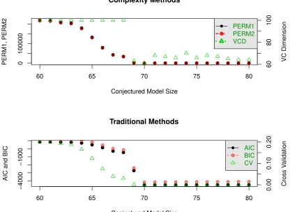
As a typical example, Fig. 1 shows the results for n = 700 and p = 70 with L = 7. When the size of the conjectured model is strictly less than the size of the true model,

ˆ

dV C is equal to the smallest design point. However, when the conjectured model exactly matches the true model, ˆdV C ≈61, underestimatingdV C. Interestingly, if we simply look at the minimal VCD value it occurs at the conjectured model of size 70, the true values ofp. When the conjectured model is more complex than the true model, the VCD value is visibly higher than the VCD value for the true model. Thus, using VCD favors parsimony more than the other methods do. In results not shown here, we increased n to 2000 and used good design points (as discussed in Subsec. 4.1.2) and found ˆdV C ≈ 70. Our observation for the other five model selection methods is that they are less affected by the small sample size, but decrease and ‘flatline’ in the sense that the AIC, BIC and CV values decrease very slowly (making it unclear which model to choose) while P ERM\ 1 and P ERM\ 2 routinely give models that are too small if one follows the usual rule of choosing the smallest local minimum. Overall, using VCD penalizes models that are too large more than other methods do, thereby giving a clearer statement about which model is true, at least in the limit with intelligently chosen design points. Other choices ofn,p, the design points, and other inputs, gave results compatible with this interpretation.

60 65 70 75 80

0

100000

PERM1, PERM2

Conjectured Model Size

60

80

100

VC Dimension

PERM1 PERM2 VCD Complexity Methods

60 65 70 75 80

−4000

−1000

AIC and BIC

Conjectured Model Size

0.00

0.10

0.20

Cross V

alidation

AIC BIC CV Traditional Methods

p = 70 , n = 700 , n_l = 100 to 700 by 100

problem with ˆdV C flatlining (or decreasing) past a certain value of dV C occurs mostly due to instability, e.g., when nis not large enough relative top.

We argue that estimating VC dimension directly is better than using P ERM\ 1 or \

P ERM2. There are several reasons. First, the computation of P ERM\ 1 and P ERM\ 2 requires ˆdV C. It also requires a threshold η be chosen (see Propositions 3 and 4) and is more dependent onm than ˆdV C is. Being more complicated than ˆdV C,P ERM\ 1,P ERM\ 2 will break down faster than ˆdV C. This is seen, for instance in tables of Mpoudeu (2017) Chap. 3 and the discussion there. More generally, we argue that P ERM\ 1, and P ERM\ 2 break down faster than ˆdV C with increasing p, if the sample size is held constant. That is,

\

P ERM1 andP ERM\ 2 are less efficient than ˆdV C.

Finally for this subsection, we reiterate our observation that in practice, when our VC dimension technique is used properly i.e., n is large enough relative to p, the σ used in Theorem 6 and the design points are adequately chosen, dˆ_VC−d_{V C}

has a well defined minimum at the true value of dV C. Also, in contrast with other methods (including using shrinkage methods to nest models) our technique is generally more sensitive to over fit, thereby giving better parsimony.

4.1.2. Dependence of dˆCV on n and NL

It is no surprise that the higher n/p is the better the discrimination of ˆdV C over models is. However, our findings are more complicated because of the design points. The informal rule is that one wants n≈10p for good parametric inference. However, this does not take into account model selection that often requiresn >10p. Indeed, for good model selection with dV C, we find that n ≥ 15 is usually sufficient, provided the design points are not badly chosen. In our examples choosing thenl’s uniformly over [0, n] generally gives decent but not optimal performance and for typical ranges of model sizes L≥ 5 will suffice even though larger values of L are usually better, say 7 ≤L ≤10. Although we are unable at this point to chracterize the tradeoff between design points and sample size, we have noted that in some cases, good choice of design points can compensate for insufficient sample size. Indeed, relatively small changes in thenl’s can have a large numerical effect whennis small; possible due to instability in the nonlinear regression step, (29).

We leave the question of optimally choosing L and thenl’s as future work even though we make the following recommendations: 1) Good choices of nl’s are spread over [0, n]. 2. More nl’s should be in [n/2, n] than in [0,n₂], but neither should be empty. 3. Good choices for nl’s tend to remain good while poor choices of nl’s may not be as damaging to inference, as n → ∞. 4. It is better to use fewer design points over a larger range than more design points over a smaller range. 5. Asnincreases thenl’s should shift upward, i.e., more in [n/2, n]. 6. If enough nl’s are large relative to p, ˆdV C may be accurate for smaller

n, perhapsn≥12p will suffice.

4.2. Analysis of a Benchmark Data Set

The goal of this section is to evaluate our method on a ‘benchmark’ data setTourobtained from the Tour de France1. We start by giving some information about Tour, then in Sec.

4.2.1 we analyze it using a model list based on two of the explanatory variables. The list is a sequence of models nested by SCAD. We evaluate our method by comparing ˆdV C to AIC, BIC, CV,P ERM\ 1, and P ERM\ 2. In Subsec. 4.2.2, we look at the effect of outliers in the estimates ˆdV C,P ERM\ 1, and P ERM\ 2.

The full data setTour hasn= 103 data points. The data points are dependent (associ-ated) because many cyclists competed in theTour de France for more than one year. Here we ignore the dependence structure because the dependencies are small enough that the complication of accounting for them is not worthwhile. Each data point has a value of the response variable (Speed), the average speed in kilometers per hour (km/h) of the winner of the Tour. The explanatory variables are the Year (Y) of the Tour and its distance (D) in kilometers. Our data is from 1903 to 2016. However, during World Wars 1 and 2 there was no Tour, so we do not have data points for those years. The effect of World War I on the speed of the winner of the tour can be seen in a scatterplot of Speed vs. Y – the lowest winning speeds were in the years just after World War I, probably due to casualties. After World War II, there was also a decrease in average winning speed, but the decrease was less than after World War I. There is a curvilinear relationship between Speed and Year and a roughly linear relationship between Speed and D; the variability of Speed increases with D.

4.2.1. Analysis of Tour Using a Nested Collection of Models

We identify a nested model list usingY, D,Y2_,D2 _{and the interaction between Year and} Distance denotedY :Das covariates. Because the size of the data set is not large, we can only use a small model list.

We order the variables using SCAD because as a shrinkage method it perturbs parameter estimates the least and satisfies an oracle property. Under SCAD, the order of inclusion of variables isY,D,D2_,Y2_{, andY :D. We therefore fit five different models. We use the six} model selection techniques from Sec. 4.1 and include ˆdV C the original estimator in Vapnik et al. (1994) for the sake of comparison. It is seen that Vapnik et al. (1994)’s original

Model dˆV dˆV C P ERM\ 1 P ERM\ 2 AIC BIC CV

Y 20 4 16.42 44.95 84 79.67 0.1294

Y, D 20 4 15.10 42.83 77 71.66 0.1209

Y, D, D2 20 4 11.21 36.37 24 26.21 0.0727

Y, D, D2_{, Y}2 _{20 4 11.09 36.16 17 28.77 0.0681}

Y, D, D2, Y2, Y :D 20 4 11.06 36.11 19 32.96 0.0691

Table 1: Model selection for the Tour de France data using seven methods. The design points for ˆdV and ˆdV C are 20, 30, 40, 50, 60, 70, 80, 90, and 100 andW = 50. So

ˆ

dV equals the smallest design point in all cases. This problem frequently occurs for ˆdV.

indicated by AIC and CV. The BIC drops the Y2 term which is not unreasonable because the curvilinearity is less than quadratic. P ERM\ 1 and P ERM\ 2 include the interaction term (which can be seen to be zero by a simple t-test). It may also be the case that the derivation of the BIC rests heavily on the independent of data which is not the case here.

4.2.2. Analysis of The Tour de France data set with outliers removed

The observations just after World War I may be outliers. So, we consider the data set formed by deleting the points from 1919 to 1926. Let us see how the six model selection techniques now behave.

The process of analyzing this reduced data set is the same: We identify the nested model lists by SCAD and then find the models corresponding to ˆdV C, AIC, BIC, CV, P ERM\ 1, and P ERM\ 2. The results are given in Table 2.

Model Size db_{V C} P ERM\ ₁ P ERM\ ₂ AIC BIC CV

Y 4 12.87 40.72 67 75 0.1181

Y,D2 4 12.01 39.26 69 79 0.1336

Y,D2,D 4 11.66 38.36 46 59 0.0919

Y,D2,D,Y2 4 11.48 38.34 28 43 0.0742

Y,D2,D,Y2,Y :D 4 11.35 38.13 29 46 0.0735

Table 2: Model selection for theTour de France data set with outliers removed.

Under SCAD, the order of inclusion of our covariates is: Y,D2,D,Y2 and Y :D. This order is different from when we used all data points. The outliers suggest Y :D was more important than it probably is. Note also that when we used all the data points, D was included before D2 and D2 was included afterY2. Again, we fit 5 nested models.

From Table 2, if we choose a model using ˆdV C, we get the same answer as in Sec. 4.2.1, the model with four variables: Y,D2,D,Y2. AIC and BIC choose the same model probably because (Y :D) has low correlation with Speed (-0.08). P ERM\ 1,P ERM\ 2 and CV choose the model of size 5, which we discount as before because Y : D is only slightly correlated with Speed. That is, the reasoning in Subsec. 4.2.1 for why we think that the model chosen by ˆdV C is best continues to hold.

4.3. Application to a Real Data Set

Our collection of explanatory variables can be grouped into three categories: phenotype, SNP, and design variables. For brevity, we fit only the phenotype variables in Subsec. 4.3.1 and phenotype plus design variables in Subsec. 4.3.2. Comparing these will show that the model selection is unaffected by the design. Also, for brevity, our only analysis is ‘multilocation’ because we pooleded the data over location-year pairs. A full analysis is in Mpoudeu and Clarke (2018).

4.3.1. Estimation of VC Dimension Using Phenotypic Covariates Only

Intuition suggests

Y IELD =β0+β1·T KW T ·KP SM+ (46)

will be a good model because YIELD is essentially the product of the number of kernels and their average weight. Likewise,

Y IELD=β0+β1·T KW T ·KP S·SP SM+ (47)

should also be a good model. So, using only phenotpic variables does not lead to aunique

good model. Both are over simplifications and we can be confident that other influences on YIELD must be considered. Indeed, a 3-dimensional plot of the vectors (YIELD, TKWT, KPSM) looks like a triangle that is bowed out to one side. The bowing means that (46) is only an approximation; other terms are required to explain YIELD. Henceforth, we focus on (46) rather than (47) because we have limited ourselves to second order models.

To implement our multilocation analysis, we first find the order of inclusion of the phenotypic variables in the model, using correlation with YIELD. Then, we find values for

ˆ

dV C, AIC, BIC, CV, P ERM\ 1, P ERM\ 2, and the models given by SCAD and ALASSO. Under absolute value of correlation with YIELD, the order of inclusion of the explanatory variables is: TKWT ·KPSM, TSTWT · KPSM, KPSM, SPSM ·KPS, KPSM2, KPSM ·

HT, TKWT·SPSM, TSTWT2, TSTWT, SPSM·KPSM, KPS·KPSM, TSTWT·SPSM, SPSM SPSM ·HT, SPSM2, TKWT ·TSTWT, TKWT, TSTWT·HT, TKWT2 TKWT·

KPS, TSTWT ·KPS, TKWT ·HT, KPS ·HT, HT, HT2 KPS, KPS2. So, we consider 27 nested models. This leads to Table 3.

First, we note there is no variability in P ERM\ 1 and P ERM\ 2 so following standard usage, they select a model with TKWT·KPSM as the only explanatory variable. Likewise, AIC, BIC, and CV suggest the one term model. However, ˆdV C = 14 means the VC dimen-sion chooses the model with the first 14 terms from the ordered list. SCAD and ALASSO both give the one term model

\

Y IELD= 3.43 + 1.12·T KW T ·KP SM, (48)

the same asP ERM\ 1,P ERM\ 2, AIC, BIC and CV. Thus the only reasonable model is the one chosen by ˆdV C.

4.3.2. Analysis of Wheat Using Phenotypic Data and the Design Structure

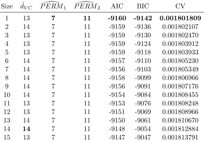
Size dˆV C P ERM\ 1 P ERM\ 2 AIC BIC CV

1 13 7 11 -9160 -9142 0.001801809

2 14 7 11 -9159 -9136 0.001802107

3 13 7 11 -9159 -9130 0.001802470

4 13 7 11 -9159 -9124 0.001803912

5 13 7 11 -9159 -9118 0.001803933

6 14 7 11 -9157 -9110 0.001805230

7 14 7 11 -9156 -9103 0.001805349

8 14 7 11 -9158 -9099 0.001806966

9 14 7 11 -9156 -9091 0.001807176

10 14 7 11 -9154 -9084 0.001808455 11 13 7 11 -9153 -9076 0.001808248 12 13 7 11 -9151 -9069 0.001808966 13 14 7 11 -9150 -9061 0.001810670 14 14 7 11 -9148 -9054 0.001812884 15 13 7 11 -9147 -9047 0.001813791

Table 3: The column labeled size gives the number of coefficients for each linear model. The 2nd through 7th columns give the corresponding estimates for ˆdV C, ERM\1,

\

ERM2, AIC, BIC, and CV for Wheat.

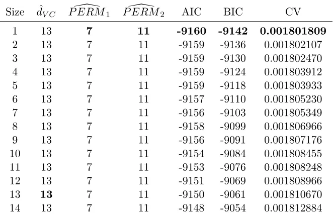
complicated bootstrap procedure that would otherwise be sufficient. Thus, to implement our method here, we perform arestrictedbootstrap. Specifically, we bootstrap in each level of the design variable (incomplete block) so that each half data set has all levels of the design structure. We do this to maintain the design structure and its effects. To include phenotypic variables in the models, we use the same order of inclusion as in Subsec. 4.3.1. The natural comparison is between Tables 3 and 4. Apart from random variation, they are identical. Moreover, the sparsity methods give exactly the same results in both settings. Thus the conclusions here are the same as in Subsec. 4.3.1: The design variables have no impact on model selection and ˆdV C gives the only plausible model.

5. Conclusions

Size dˆV C P ERM\ 1 P ERM\ 2 AIC BIC CV

1 13 7 11 -9160 -9142 0.001801809

2 13 7 11 -9159 -9136 0.001802107

3 13 7 11 -9159 -9130 0.001802470

4 13 7 11 -9159 -9124 0.001803912

5 13 7 11 -9159 -9118 0.001803933

6 13 7 11 -9157 -9110 0.001805230

7 13 7 11 -9156 -9103 0.001805349

8 13 7 11 -9158 -9099 0.001806966

9 13 7 11 -9156 -9091 0.001807176

10 13 7 11 -9154 -9084 0.001808455 11 13 7 11 -9153 -9076 0.001808248 12 13 7 11 -9151 -9069 0.001808966 13 13 7 11 -9150 -9061 0.001810670 14 13 7 11 -9148 -9054 0.001812884

Table 4: The column labeled size gives the number of coefficients for each linear model. The 2nd through 7th columns give the corresponding estimates for ˆdV C,P ERM\ 1,

\

P ERM2, AIC, BIC, and CV for multi-location analysis with design structure.

We have done an extensive comparison of our estimator of VC dimension as a model selection method with seven established model selection methods, namely two forms of empirical risk minimization, AIC, BIC, CV, and two sparsity criteria. Other examples can be found in Mpoudeu and Clarke (2018). We did this for the special case of linear models but the same reasoning can be used for any class of nonlinear models e.g., trees, for which the VC dimension can be identified. We also gave one example of how our estimator for VC dimension performs better than the original estimator in Vapnik et al. (1994). As a generality, our method equals or outperforms these other methods.

Acknowledgments

The authors gratefully acknowledge support from NSF grant # DMS-1419754 and invalu-able computational support from the Holland Computing Center. Data, code, and results for the full versions of the analyses presented here can be found at https://github.com/ poudas1981/Wheat_data_set. We also express our gratitude to a sophisticated and hard-working referee and Editor who helped us improve our work immensely.

References

M. Anthony and P. Bartlett. Neural network learning: Theoretical foundations. Cambridge University Press, 2009.

A. Barron and T. Cover. Minimum complexity density estimation. IEEE Transactions on

J. Bernardo and A. F. M. Smith. Bayesian Theory. Wiley Series in Probability and Statis-tics, 2000.

B. Campbell, P. Baenziger, P. Stephen, K. Gill, K. Eskridge, H. Budak, M. Erayman, I. Dweikat, and Y. Yen. Identification of qtls and environmental interactions associated with agronomic traits on chromosome 3a of wheat. Crop Science, 43:1493–1505, 2003. P. Dhungana, K. Eskridge, P. Baenziger, B. Campbell, K. Gill, and I. Dweikat. Analysis

of genotype-by-environment interaction in wheat using a structural equation model and chromosome substitution lines. Crop Science, 47:477–484, 2007.

M. Dilbirligi, M. Erayman, B. Campbell, H. Randhawa, P. Baenziger, I. Dweikat, and K. Gill. High-density mapping and comparative analysis of agronomically important traits on wheat chromosome 3a. Genomics, 88:74 – 87, 2006. ISSN 0888-7543. doi: https:// doi.org/10.1016/j.ygeno.2006.02.001. URL http://www.sciencedirect.com/science/ article/pii/S0888754306000437.

J. Fan and R. Li. Variable selection via nonconcave penalized likelihood and its oracle prop-erties. Journal of the American Statistical Association, 96(456):1348–1360, 2001. doi: 10. 1198/016214501753382273. URLhttp://dx.doi.org/10.1198/016214501753382273.

J. Fan and J. Lv. Sure independence screening for ultrahigh dimensional feature space.

Journal of the Royal Statistical Society: Series B (Statistical Methodology), 70(5):849–

911, 2008.

D. McDonald, C. Shalizi, and M. Schervish. Estimated VC dimension for risk bounds. preprint arXiv:1111.3404, 2011.

M. Mpoudeu. Use of Vapnik-Chervonenkis Dimension in Model Selection. PhD thesis, University of Nebraska-Lincoln, 2017. See: https://arxiv.org/pdf/1808.06684.pdf.

M. Mpoudeu and B. Clarke. Model selection via the VC dimension. See: https: // arxiv. org/ abs/ 1808. 05296, 2018.

K. Murphy. Machine Learning: A Probabilistic Perspective. The MIT Press, 2012.

X. Shao, V. Cherkassky, and W. Li. Measuring the VC dimension using optimized experi-mental design. Neural computation, 12(8):1969–1986, 2000.

V. Vapnik. Statistical Learning Theory. Wiley, New York, 1998.

V. Vapnik and A. Chervonenkis. On the uniform convergence of relative frequencies of events to their probabilities. In Soviet Math. Dokl, volume 9, pages 915–918, 1968. V. Vapnik and A. Chervonenkis. On the uniform convergence of relative frequencies to their

probabilities. In Soviet Math. Dokl, volume 9, pages 915–918, 1971.

V. Vapnik, E. Levin, and Y. LeCun. Measuring the VC dimension of a learning machine.

Neural Computation, 6(5):851–876, 1994.

H. Zou. The adaptive lasso and its oracle properties. Journal of the American Statistical