146
Copyright © 2017. Vandana Publications. All Rights Reserved.
Volume-7, Issue-6, November-December 2017
International Journal of Engineering and Management Research
Page Number: 146-151
Modeling Contemporaneous and Causal Relationships of Stock Trading
Variables (Case Study of Indonesian Stock Exchange on LQ-45 Index)
N. Valentika1, E.H. Nugrahani2, D. C. Lesmana3
1,2,3Department of Mathematics, Bogor Agricultural University, INDONESIA
ABSTRACT
A variable value may be affected by variable another at the same period. However, a variable may also be affected by itself or other variable at different period of time. This paper presents modification of Paital and Sharma model [12] by adding the return variable on Indonesian stock data with case study of LQ-45 Index. This paper empirically examines the relationship among trading volume, bid-ask spread, volatility and stock return. Regression results show that there are weak contemporaneous relationship between stock trading variables. Thus, it indicates that Indonesian market is inefficient. Based on Granger causality test, it is found that LQ-45 intraday stock sample trading tend to follow the mixture of distribution hypothesis theory.
Keywords— Contemporaneous and causal relationship, stocks
I.
INTRODUCTION
The capital market is defined as a market for trading securities that generally have more than one year time horizon, such as stocks and bonds [14]. In capital market, there are several trading assets such as stocks and bonds. In this paper, stock is taken as the trading asset. There are many variables that determined the price of stocks, i.e. bid-ask spread, trading volume, volatility and stock return. Among the various variables there could be possibility of the presence of contemporaneous relationship among variables, where a variable value is affected by another at the same period. However, a variable may also be affected by itself or other variable at different period of time [1]. In theoretical level, the existence of such positive relationship explained mainly by two major underlying hypotheses; the mixture of distribution hypothesis (MDH) and the sequential information arrival hypothesis (SIAH) [12]. In economics, relationship between risk and expected return are in the same direction and linear [14].
The mixture of distribution hypothesis developed by Clark (1973) implies that the volume-volatility relationship is dependent upon the rate of information flow into the market. The theory assumes that
new price signals is received by all traders simultaneously and immediately shift to a new equilibrium. Thus, both volatility and volume change contemporaneously in response to the arrival of new information [8]. The mixture of distribution hypothesis supports only positive contemporaneous relationship, but no causal linkage between trading volume and volatility occurs [12].
The sequential information arrival hypothesis developed by Copeland (1976), Jennings, Starks and Fellingham (1981) [8]. According to this model, new information is disseminated sequentially rather than simultaneously to all traders [12]. In these models, some trader observes a signal ahead of the market and trades on it, thereby creating volume and price volatility. As a result, volatility and volume move in the same direction. Therefore, there is a positive contemporaneous relationship between volatility and volume. Smirlock and Starks (1988) have further extended the hypothesis that as information comes sequentially, the past values of trading volume may have the ability to predict future volatility and vice versa, which means that a causal relationship may exist in either directions between volatility and trading volume [12].
Paital and Sharma’s research [12] analyze the contemporaneous and causal relationships between bid-ask spread, trading volume and volatility in Indian stock market. Parameter estimating method in Paital and Sharma’s research [12] is the ordinary least square (OLS). Paital and Sharma’s research [12] was consistent with the sequential information arrival hypothesis and contradicts the mixture of distribution hypothesis in Indian stock market.
This paper use contemporaneous and causal relationships model between trading variables from Paital and Sharma’s research [12] and add a contemporaneous and causality relationship model between stock return and volatility.
II.
DATA AND VARIABLES
DESCRIPTION
147
Copyright © 2017. Vandana Publications. All Rights Reserved.
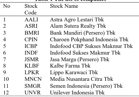
ARCH effect in the residual of the constant averageequation model and satisfying GARCH (1,0) or GARCH (1,1). Table 1 provides the list of companies.
Table 1 The list of companies
No Stock Code
Stock Name
1 AALI Astra Agro Lestari Tbk 2 ASRI Alam Sutera Realty Tbk 3 BMRI Bank Mandiri (Persero) Tbk 4 CPIN Charoen Pokphand Indonesia Tbk 5 ICBP Indofood CBP Sukses Makmur Tbk 6 INDF Indofood Sukses Makmur Tbk 7 JSMR Jasa Marga (Persero) Tbk 8 KLBF Kalbe Farma Tbk 9 LPKR Lippo Karawaci Tbk 10 MNCN Media Nusantara Citra Tbk 11 SMGR Semen Indonesia (Persero) Tbk 12 UNVR Unilever Indonesia Tbk
Our primary data set consists of the close price, trading volume, and the close bid and ask price using intraday intervals from 3 August 2015 to 29 July 2016 for all stocks. All the data are obtained electronically from www.idx.co.id.
Trading variables are defined as a. Return at time t
(
⁄ )
where represents closed price at time t.
b. Bid-Ask Spread is difference between ask and bid price. The proportional intraday bid-ask spread at time
t
[ ]
c. Volatility is estimated using GARCH model. Initialization of the variation in GARCH estimation in this paper is assumed to using a fixed method, that is the square of the residual (return) of the previous observation following [5], [7], and [11].
d. Trading Volume is defined as
where is trading volume at time t. Following [12], this paper uses logarithmic value of volume instead of raw volume to improve the normality properties of the series.
III. CONTEMPORANEOUS AND
CAUSAL MODELS
This paper presents the models contemporaneous and causal relationships between trading variables.
The contemporaneous model presented in this paper are
a. Contemporaneous relationship between volatility and trading volume
(3.1) b. Contemporaneous relationship between volatility and
bid-ask spread
(3.2) c. Contemporaneous relationship between volatility and
stock return
(3.3) where and are stock return, volatility, trading volume and bid-ask spread respectively at time t.
The pair wise causality between stock trading variables are given by the following unrestricted equations:
a. The causal relationship between bid-ask spread and volatility
∑
∑
(3.4)
∑
∑
(3.5)
b. The causal relationship between stock return and volatility
∑
∑
(3.6)
∑
∑
(3.7)
c. The causal relationship between trading volume and volatility
∑
∑
(3.8)
∑
∑
(3.9)
where is intercept, is parameter and is the optimal lag length, where , and .
In the causal relationship between trading volume and volatility, we formulate the linear Granger causality restrictions as follows: If some of values are statistically not equal to zero, then trading volume is said to Granger cause volatility, which is the main hypothesis of interest. Similarly if some of values are statistically not equal to zero, then volatility are said to Granger cause volume. If both and are statistically significant then a feedback relationship is said to exist. Similarly we checked the causality among volatility, bid-ask spread and stock return.
Determination of the optimal lag length is carried out by observing at the lag that has the biggest
Likelihood Ratio (LR) value, and the smallest of all Final Prediction Error (FPE), Akaike Information Criterion
148
Copyright © 2017. Vandana Publications. All Rights Reserved.
IV. IMPLEMENTATION RESULTS
4.1 Cross-Correlation
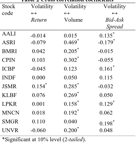
One of the measures being used in relationship analysis is correlation coefficient. The correlation coefficient used is Pearson correlation coefficient. The result of the correlation coefficients are presented in Table 2.
Table 2 Cross correlation coefficients
Stock code
Volatility ↔
Return
Volatility ↔ Volume
Volatility ↔
Bid-Ask Spread
AALI -0.014 0.015 0.135*
ASRI -0.079 0.469* -0.179* BMRI 0.042 0.205* -0.015
CPIN 0.103 0.302* -0.055 ICBP -0.045 0.123 0.161*
INDF 0.000 0.050 0.115 JSMR 0.154* 0.285* -0.032
KLBF 0.076 0.269* 0.050 LPKR 0.001 0.158* 0.129*
MNCN 0.018 0.192* 0.062 SMGR 0.110 0.040 0.198*
UNVR -0.060 0.200* 0.048
*Significant at 10% level (2-tailed).
According to Table 2, there is positive relationship between volatility and stock return for all stocks except AALI, ASRI, ICBP, INDF and UNVR. There is positive relationship between volatility and trading volume for all stocks. Based on correlation coefficient, the relationship between volatility and trading volume is positive but relatively weak. It was shown by the low correlation coefficient in all stocks. There is positive relationship between volatility and bid-ask spread for all stocks except ASRI, BMRI, CPIN, and JSMR.
4.2 Contemporaneous Relationship Model
Contemporaneous relationship model is used after basic classic regression assumption test for simple linear regression, such as autocorrelation and heteroscedasticity conducted. The test being used to detect autocorrelation assumption violation in regression equation is Breusch-Godfrey Test. The test being used to detect heteroscedasticity assumption violation in regression equation is Breusch-Pagan-Godfrey. In this paper, Cochrane-Orcutt is the method being used to overcome assumption violation if autocorrelation assumption violation. White heteroscedasticity-consistent standard error & covariance is the method being used to overcome violation on non-heteroscedasticity assumption. Contemporaneous relationship between volatility and trading volume
Model of contemporaneous relationship between volatility and trading volume is given in equation (3.1).
Results of contemporaneous relationship between volatility and trading volume are presented in Table 3. The parameter measures the contemporaneous relationship between volatility and trading volume. A statistically significant and positive value of would indicate a positive contemporaneous relationship between volatility and trading volume.
Table 3 Contemporaneous relationship between volatility and trading volume
Stock code
R-squared
AALI 0.005273* -0.000913* 0.027173 ASRI 0.007227* 3.98E-05 0.000022 BMRI 0.000680 0.001232* 0.016739 CPIN 0.003637* -0.000407 0.005084 ICBP 0.005265* -0.000358 0.002358 INDF 0.000693* -0.000284* 0.017557 JSMR -0.009324 0.001995* 0.081037 KLBF -0.008166 0.001893* 0.052173 LPKR -0.001214 0.001272* 0.025000 MNCN 0.006354* -0.001008* 0.035103 SMGR 0.000839* -0.000586* 0.023854 UNVR 0.007901* 0.000155 0.000292 *Significant at 10% level.
According to Table 3, it is found that BMRI, JSMR, KLBF and LPKR stocks have positive contemporaneous relationship between trading volume and volatility which statistically significant at 10% level. AALI, INDF, MNCN and SMGR stocks have negative contemporaneous relationship between trading volume and volatility which statistically significant at 10% level. ASRI, CPIN, ICBP and UNVR stocks do not have contemporaneous relationship between trading volume and volatility which is shown by statistically insignificant of value.
The regression results also show that the positive contemporaneous volume explains a relatively small portion of volatility as shown by the low R-squared values in BMRI, JSMR, KLBF, and LPKR stocks. The weak positive contemporaneous relationship indicates that Indonesian market is informationally inefficient. The flow of information in the market may well be disseminated sequentially rather than simultaneously as required in MDH. This relationship indicates that the information flows sequentially in Indonesian market. Contemporaneous relationship between volatility and bid-ask spread
Model of contemporaneous relationship between volatility and bid-ask spread is given in equation (3.2). Results of contemporaneous relationship between volatility and bid-ask spread are presented in Table 4. The parameter measures the contemporaneous relationship between bid-ask spread and volatility.
Table 4 Contemporaneous relationship between volatility and bid-ask spread
Stock code R-squared
149
Copyright © 2017. Vandana Publications. All Rights Reserved.
ASRI 0.007982* -0.206421 0.003392BMRI 0.015508* -0.081903 0.001597 CPIN 0.001691* -0.032259 0.004852 ICBP 0.004840* -0.068032 0.013761 INDF 0.000901* -0.060907* 0.046814 JSMR 0.018056* -0.090327 0.003575 KLBF 0.018890* 0.054886 0.001880 LPKR 0.018267* 0.129044* 0.012527 MNCN 0.004043* 0.045684 0.009113 SMGR 0.001567* 0.010976 0.000436 UNVR 0.008300* -0.128959* 0.021418 *Significant at 10% level.
According to Table 4, it is found that LPKR stock has positive contemporaneous relationship between bid-ask spread and volatility which statistically significant at 10% level. INDF and UNVR stocks have negative contemporaneous relationship between bid-ask spread and volatility which statistically significant at 10% level. AALI, ASRI, BMRI, CPIN, ICBP, JSMR, KLBF, MNCN and SMGR stocks do not have contemporaneous relationship between bid-ask spread and volatility which is shown by statistically insignificant of value.
The regression results show that contemporaneous bid-ask spread explains a relatively small portion of volatility as shown by low R-squared values. So this relationship indicates that the information flows sequentially in Indonesian market.
Contemporaneous relationship between volatility and return
Model of contemporaneous relationship between volatility and returnis given in equation (3.3). Results of contemporaneous relationship between volatility and return are presented in Table 5. The parameter measures the contemporaneous relationship between volatility and return.
Table 5 Contemporaneous relationship between volatility and return
Stock code
R-squared
AALI 0.003568* -0.020278* 0.050182 ASRI 0.007571* -0.017328* 0.016813 BMRI 0.015343* 0.006827 0.001204 CPIN 0.001856* 0.004161 0.003191 ICBP 0.003547* -0.047595* 0.093828 INDF 0.000549* 0.001147 0.001064 JSMR 0.018501* 0.025638* 0.015057 KLBF 0.019675* 0.001873 0.000128 LPKR 0.018541* 0.001890 0.000115 MNCN 0.004110* -0.010554 0.018897 SMGR 0.000863* 0.000268 0.000024 UNVR 0.007448* -0.043831* 0.069608 *Significant at 10% level.
According to Table 5, it is found that JSMR stock has positive contemporaneous relationship between stock return and volatility which statistically significant at 10% level. AALI, ASRI, ICBP, and UNVR have negative contemporaneous relationship between stock return and
volatility which statistically significant at 10% level. BMRI, CPIN, INDF, KLBF, LPKR, MNCN and SMGR do not have contemporaneous relationship between stock return and volatility which is shown by statistically insignificant of value.
The regression results show that contemporaneous stock return explains a relatively small portion of volatility as shown by low R-squared values. So this relationship indicates that the information flows sequentially in Indonesian market.
4.3 Granger Causality Models
In reality the characteristic of economic variable has not only one way relationship but also two-way relationship which is known as causality concept. This causal relationship can be tested using Granger causality test [10]. Granger causality test can be meaningless if it involves nonstationary variables. In other words, Granger causality involves only stationary variables [4].
Stationarity Test
Problems which often occur in time series data are nonstationary data. The data needs special treatment to be applied in time series analysis. This is caused by the potential of spurious regression results [6]. ADF test is a formal test to check whether the data is stationary or not. The results of data stationary test show that the variables are stationary in level at 10% level in all stocks except for the trading volume of MNCN stock. Trading volume variable of MNCN stock is not stationary in level, but stationary in first difference (order 1).
Granger Causal Relationship between Bid-Ask Spread and Volatility
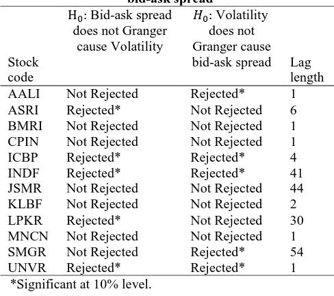
The causal relationship models between bid-ask spread and volatility are presented in equation (3.4) and equation (3.5). Because bid-ask spread and volatility are stationary in level for all stocks, then bid-ask spread and volatility used for Granger causality test is time series data integrated with order zero or written as I(0). The result of Granger causality test in bid-ask spread and volatility relationship is presented in Table 6.
Table 6 Granger causality test between volatility and bid-ask spread
Stock code
Bid-ask spread does not Granger
cause Volatility
Volatility does not Granger cause bid-ask spread Lag
length AALI Not Rejected Rejected* 1 ASRI Rejected* Not Rejected 6 BMRI Not Rejected Not Rejected 1 CPIN Not Rejected Not Rejected 1 ICBP Rejected* Rejected* 4 INDF Rejected* Rejected* 41 JSMR Not Rejected Not Rejected 44 KLBF Not Rejected Not Rejected 2 LPKR Rejected* Not Rejected 30 MNCN Not Rejected Not Rejected 1 SMGR Not Rejected Rejected* 54 UNVR Rejected* Rejected* 1
150
Copyright © 2017. Vandana Publications. All Rights Reserved.
According to Table 6, bid-ask spreadsignificantly affects volatility for ASRI, ICBP, INDF, LPKR, and UNVR stocks at 10% level. Volatility significantly affects bid-ask spread for AALI, ICBP, INDF, SMGR, and UNVR stocks at 10% level. Therefore there are two-way causal relationship between bid-ask spread and volatility for ICBP, INDF, and UNVR stocks. Granger Causal Relationship between Stock Return and Volatility
The causal relationship models between stock return and volatility are presented in equation (3.6) and equation (3.7). Because stock return and volatility are stationary in level for all stocks, then stock return and volatility used for Granger causality test is time series data integrated with order zero or written as I(0). The result of Granger causality test in stock return and volatility relationship is presented in Table 7.
According to Table 7, stock return significantly affects volatility for all stocks except BMRI and JSMR at 10% level. Volatility significantly affects stock return for SMGR and CPIN stocks at 10% level. Therefore there are two-way causal relationship between stock return and volatility for CPIN and SMGR stocks.
Table 7 Granger causality test between Volatility and Stock Return
Stock code
Stock return does not Granger cause
Volatility
Volatility does not Granger cause
stock return Lag length AALI Rejected* Not Rejected 1 ASRI Rejected* Not Rejected 25 BMRI Not Rejected Not Rejected 43 CPIN Rejected* Rejected* 5 ICBP Rejected* Not Rejected 1 INDF Rejected* Not Rejected 37 JSMR Not Rejected Not Rejected 62 KLBF Rejected* Not Rejected 1 LPKR Rejected* Not Rejected 41 MNCN Rejected* Not Rejected 1 SMGR Rejected* Rejected* 41 UNVR Rejected* Not Rejected 1 *Significant at 10% level.
Granger Causal Relationship between Trading Volume and Volatility
The causal relationship models between trading volume and volatility are presented in equation (3.8) and equation (3.9). Because trading volume and volatility are stationary in level for all stocks except MNCN stock, then trading volume and volatility used for Granger Causality test is time series data integrated with order zero or written as I(0) for all stocks except MNCN stock. Trading volume in MNCN stock is not stationary in level, but it is stationary in first difference (order 1).
Therefore trading volume and volatility used in the Granger causality test for MNCN stock are time series data integrated with order 1 or written as I(1). The result
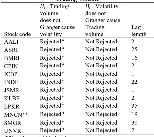
of Granger causality test in trading volume and volatility relationship is presented in Table 8.
Table 8 Granger causality test between Volatility and Trading Volume
Stock code
Trading volume does not Granger cause volatility
Volatility does not Granger cause Trading volume
Lag length AALI Rejected* Not Rejected 2 ASRI Rejected* Not Rejected 25 BMRI Rejected* Not Rejected 16 CPIN Rejected* Not Rejected 21 ICBP Rejected* Not Rejected 1 INDF Rejected* Not Rejected 22 JSMR Rejected* Not Rejected 1 KLBF Rejected* Not Rejected 2 LPKR Rejected* Not Rejected 35 MNCN** Rejected* Not Rejected 19 SMGR Rejected* Not Rejected 30 UNVR Rejected* Not Rejected 2
*Significant at 10% level.
**Using trading volume data and volatility in first difference.
According to Table 8, trading volume significantly affects volatility for all stocks at 10% level. Volatility does not affect trading volume for all stocks. Because there are one-way relationship between trading volume and volatility for all stocks, then there is insufficient evidence to support the validity of SIAH theory. Insufficient evidence to support the existence of SIAH theorygives an assumption that the LQ-45 stock sample in the intraday trade tends to follow MDH theory.
V. CONCLUSION
The implementation of contemporaneous models show that there is weak positive contemporaneous relationship between trading volume and volatility in BMRI, JSMR, KLBF, and LPKR stocks. This indicates that the flow of information in the market are disseminated sequentially rather than simultaneously as required by MDH. Moreover, the results show that there are weak contemporaneous relationship between bid-ask spread, stock return and trading volume with volatility. Thus, these relationships indicate that the information flow sequentially in Indonesian market.
151
Copyright © 2017. Vandana Publications. All Rights Reserved.
LQ-45 stock sample in the intraday trading tends tofollow MDH theory.
REFERENCES
[1] Ariefianto MD. 2012. Ekonometrika Esensi dan Aplikasi dengan menggunakan EViews. Jakarta (ID): Erlangga.
[2] Clark, P. (1973). A subordinated stochastic process model with finite variance for speculative prices.
Econometrica, 41, 135-155.
[3] Copeland, T. (1976). A model of asset trading under the assumption of sequential information arrival. Journal of Finance, 31. 1149-1168.
[4] Enders W. 2015. Applied Econometric Time Series. New York: John Wiley and Sons, Inc.
[5] Engle RF, Patton AJ. 2001. What good is a volatility model? Quantitative Finance 1, 237-245.
[6] Granger CWJ, Newbold P. 1974. Spurious regressions in econometrics. Journal of Econometrics, Vol. 2. 111-120.
[7] Hull JC. 2012. Options, futures, and other derivatives. Boston (US): Prentice Hall.
[8] Hussain, SM. 2011. The Intraday Behaviour of Bid-Ask Spreads, Trading Volume, and Return Volatility: Evidence from DAX 30. International Journal of Economics and Finance. 3(1):23-34.
[9] Jennings, R., Starks, L. & Fellingham, J. (1981). An equilibrium model of asset trading with sequential information arrival. Journal of Finance, 36. 143-162. [10] Juanda B, Junaidi. 2012. Ekonometrika Deret Waktu. Bogor (ID): IPB Press.
[11] Lo MS. 2000. Generalized Autoregressive Conditional Heteroscedastic Time Series Models. Simon Fraser University.
[12] Paital RR, Sharma NK. 2016. Bid-Ask Spreads, Trading Volume and Return Volatility. Eurasian Journal of Economics and Finance. 4(1):24-40.
[13] Smirlock, M. and Starks, L., 1988. An empirical analysis of the stock price-volume relationship. Journal of Banking and Finance, 12. 31-41.