The Thirty-Third AAAI Conference on Artificial Intelligence (AAAI-19)
Plan-Length Bounds: Beyond 1-Way Dependency
Mohammad Abdulaziz
Technical University of Munich, Munich, Germany
Abstract
We consider the problem of compositionally computing up-per bounds on lengths of plans. Following existing work, our approach is based on a decomposition of state-variable de-pendency graphs (a.k.a. causal graphs). Tight bounds have been demonstrated previously for problems where key de-pendencies flow in a single direction—i.e. manipulating vari-ablev1can disturb the ability to manipulatev2andnotvice
versa. We develop a more general bounding approach which allows us to compute useful bounds where dependency flows in both directions. Our approach is practically most useful when combined with earlier approaches, where the computed bounds are substantially improved in a relatively broad vari-ety of problems. When combined with an existing planning procedure, the improved bounds yield coverage improve-ments for both solvable and unsolvable planning problems.
Introduction
Many techniques for solving reachability problems in tran-sition systems, like SAT-based planning (Kautz and Selman 1992) and bounded model checking (Biere et al. 1999), ben-efit from knowledge ofupper boundson the lengths of tran-sition sequences, akacompleteness thresholds. IfNis such a bound, and if a transition sequence achieving the goal exists, then that sequence need not comprise more thanN actions.
Biere et al. (1999) identify the diameter and the re-currence diameter, which are topological properties of the state space, as conceptually appealing upper bounds. The diameter is the longest shortest path between any two states. The recurrence diameter is the longest simple path in the state space, i.e. the longest path that does not tra-verse any state more than once. Approximate and exact algorithms have been developed to calculate both proper-ties given an explicit (e.g. tabular) representation of the transition system. Exact algorithms to compute the diam-eter have worse than quadratic runtimes in the number of states (Fredman 1976; Alon, Galil, and Margalit 1997; Chan 2010; Yuster 2010), and approximation approaches have super-linear runtimes (Aingworth et al. 1999; Roditty and Vassilevska Williams 2013; Chechik et al. 2014; Ab-boud, Williams, and Wang 2016). The situation is even worse for the recurrence diameter, whose computation is
Copyright c2019, Association for the Advancement of Artificial Intelligence (www.aaai.org). All rights reserved.
NP-Hard (Pardalos and Migdalas 2004). The impractical-ity of those explicit algorithms is exacerbated in settings where systems are described using factored representations, like planning and model-checking, since a system’s explicit representation can be exponential in the size of the corre-sponding factored problem description.
However,compositionalapproaches to calculate bounds for problems described using factored representations are feasible. The concrete system’s (recurrence) diameter is bounded by composing together bounds for abstract subsys-tems. The subsystems are projectionsof the concrete sys-tem. The motivation for compositional approaches is that they provide useful approximations of plan bounds using smaller computational effort, since only explicit representa-tions of abstract subsystems have to be constructed. Baum-gartner, Kuehlmann, and Abraham (2002) and Rintanen and Gretton (2013) followed this projection-based approach to develop procedures to compositionally bound the diameter. This was later improved by Abdulaziz, Gretton, and Nor-rish (2015) and Abdulaziz, Gretton, and NorNor-rish (2017) (we refer to those two papers as AGN1 and AGN2 hereafter).
A common drawback with previous approaches, how-ever, is that they are only usefully applicable if the pro-jections are induced by acyclicity in the causal/dependency graph (Williams and Nayak 1997; Knoblock 1994). Thus it is an open question as to whether there are practically useful ways to upper-bound plan lengths using projections not re-sulting from dependency graphs with acyclicity. We address this question by developing a compositional bounding pro-cedure which is applicable to arbitrary projections. We do so by defining a new topological property for the state space to which we refer as thetraversal diameter. The distinctive feature of the traversal diameter is that, for any given fac-tored transition system, the traversal diameter of that system is upper bounded by the product of the traversal diameters of projections of that system. Those projections can be ob-tained using any partition of the system’s state variables, i.e. the restriction of having acyclic dependencies is not required for this compositional bound.
state-of-the-art algorithms from AGN1 and AGN2. We use the traversal diameter based method to further decompose “atomic sub-problems”, which are abstractions that cannot be further abstracted by the algorithms from AGN1 and AGN2. We experimentally show that this additional decom-position improves the bounds computed by the algorithms from AGN1 and AGN2. For instance, bounds computed us-ing the method from AGN2 improved in 68% of the plannus-ing problems on which we experimented, with an improvement of at least 50% in 71% of the cases.
We also use the bounds computed by the new algorithm as horizons for the SAT-based planner Madagascar MP (Rinta-nen 2012). This improves the coverage of MPin both solv-able and unsolvsolv-able planning instances compared to the de-fault query strategies or to upper bounds computed by all previous algorithms as horizons.
Background and Notations
Compositional bounds are defined on factored transition systemswhich are purely characterised in terms of a set of actions. From actions we can define a set ofvalid states, and then approach bounds by considering properties of execu-tionsof actions on valid states. Whereas conventional expo-sitions in the planning and model-checking literature would also define initial conditions and goal/safety criteria, here we omit those features from discussion since the notion of diameter and other bounds are independent of those features.
Definition 1(States and Actions). A maplet,v 7→ b, maps a variablev—i.e. a state-characterising proposition—to a Booleanb. A state,x, is a finite set of maplets. We writeD(x) to denote{v | (v 7→ b) ∈ x}, the domain ofx. For states x1andx2, the union,x1]x2, is defined as{v 7→b |v ∈ D(x1)∪ D(x2)∧ifv ∈ D(x1)then b=x1(v)elseb =
x2(v)}. Note that the statex1takes precedence. An action
is a pair of states,(p, e), whereprepresents the precondi-tionsanderepresents theeffects. For actionπ= (p, e), the domain of that action isD(π)≡ D(p)∪ D(e).
Definition 2(Execution). When an actionπ (= (p, e))is executed at statex, it produces a successor stateπ(x), for-mally defined asπ(x) = if p* xthen x else e]x. We lift execution to lists of actions→π, so→π(x)denotes the state resulting from successively applying each action from→π in turn, starting atx.
We give examples of states and actions using sets of lit-erals. For example, {a, b} is a state where state variables a is (maps to) true, b is false, and its domain is {a, b}.
({a, b},{c})is an action that if executed in a state that hasa andb, it setscto true.D(({a, b},{c})) ={a, b, c}.
Definition 3(Factored Transition System). A set of actions δconstitutes a factored transition system.D(δ)denotes the domain of δ, which is the union of the domains of all the actions it contains. Letset(→π)be the set of elements from→π. The set of valid action sequences,δ∗, is{→π| set(→π)⊆δ}. The set of valid states,U(δ), is{x | D(x) = D(δ)}.G(δ)
denotes the state space ofδ, i.e. the digraph whose vertices areU(δ)and edges are{(x, π(x))|x∈U(δ), π∈δ}.
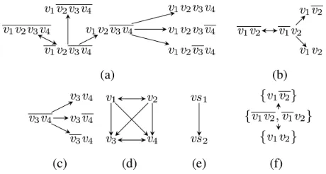
Figure 1: a) is the largest connected component of the state space ofδin Example 1. b) and c) are the state spaces of the projections of δon{v1,v2}and{v3,v4}. d) is the
depen-dency graphGD(δ)ofδand e) is a lifted dependency graph GVSforδ. f) is a quotient of the state space ofδvs1.
Example 1. Consider the factored representation, δ =
{π1 = ({v1,v2},{v2}), π2 = ({v1,v2},{v2}), π3 = ({v1,
v2},{v1,v2}), π4 = ({v1,v2},{v1}), π5 = ({v1,v2,v3,
v4},{v4}), π6 = ({v1,v2,v3,v4},{v3}), π7 = ({v1,v2,
v3,v4},{v3,v4})}. The digraph in Figure 1a represents the
largest connected component in the state space ofδ, where different states defined on the variablesD(δ) = {v1,v2v3,
v4} are shown. Interpreting δ as a transition system, it has two “modes” of operation. The first mode changes the assignments of {v1,v2} and is represented by actions {π1· · ·π4}. The second mode, represented by actions{π5,
π6, π7}, changes the assignments of{v3,v4}and is only
en-abled if{v1,v2}are both set to true.
Compositional Bounding
For a systemδ, a bound on the length of action sequences is EXP(δ) = 2|D(δ)|−1 (i.e. one less than the size of the
state space), where| • | denotes the cardinality of a set or the length of a list. Other bounds employed by previous ap-proaches are topological properties of the state space like the diameter, suggested by Biere et al. 1999.
Definition 4(Diameter). The diameter, writtend(δ), is the length of the longest shortest action sequence, formally
d(δ) = max
x∈U(δ),→π∈δ∗
min
→
π(x)=→π0(x),→π0∈δ∗
|→π0|
Note that if there is a valid action sequence between any two states, then there is a valid action sequence between them which is no longer than the diameter. Another topo-logical property suggested by Biere et al. 1999 as a suitable upper bound is the recurrence diameter.
Definition 5(Recurrence Diameter). Letdistinct(x,→π) de-note that all states traversed by executing→πatxare distinct states. The recurrence diameter is the length of the longest simple path in the state space, formally
rd(δ) = max
x∈U(δ),→π∈δ∗,distinct(x,→π)
Choosing a topological property as an upper bound de-pends on many factors. Size: for a systemδ, d(δ)can be exponentially smaller thanrd(δ), which in turn can be expo-nentially smaller than EXP(δ)(Biere et al. 1999). Complex-ity: computing EXP(δ)is the easiest since it can be done in a time linear in|D(δ)|, while the diameter can be computed in time at least quadratic in the size of the state space (Ab-boud, Williams, and Wang 2016), and the recurrence diam-eter is the hardest as it is NP-Hard in the size of the state space (Pardalos and Migdalas 2004).Usability: the diame-ter is a completeness threshold for SAT-based AI planning and bounded model checking of safety formulae, while the recurrence diameter is a completeness threshold for bounded model checking of fairness formulae (Biere et al. 1999).
In this work, the most relevant trait of a topological prop-erty is the ability to compositionally bound it. By that we mean computing an upper bound on the topological prop-erty of a given system by composing topological properties of abstractions of that system. A key abstraction concept for compositional reasoning about transition systems is projec-tion, which is defined as follows.
Definition 6(Projection). Projecting an object (a statex, an actionπ, a sequence of actions→πor a factored represen-tationδ) on a set of variablesvsrestricts the domain of the object or the components of composite objects tovs. Pro-jection is denoted asxvs,πvs,→πvs andδvs for a state, action, action sequence and factored representation, respec-tively. However, for action sequences or transition systems, an action with no effects after projection is droppedentirely. Example 2. Letvs1={v1,v2}andvs2={v3,v4}. A
par-tition of the domain ofδfrom Example 1 is{vs1,vs2}. The
projectionδvs
2 = {π5vs2 = ({v3,v4},{v4}), π6vs2 = ({v3,v4},{v3}), π7vs2 = ({v3,v4},{v3,v4})}. The vari-ables{v1,v2}were removed from action preconditions and
effects, and actions with empty effects were removed. Fig-ures 1b and 1c show the state spaces of the projectionsδvs1 andδvs2.
Compositional techniques that use projection bound a topological property of a systemδ by topological proper-ties of a set of projections ofδ. Those projections are done on a partitionvs1..n of the set of state variables D(δ). For
instance, for any vs1..n, EXP(δ) is equal to (and
accord-ingly bounded by)
Π
vs∈vs1..n(EXP(δvs) + 1)−1, i.e. theproduct of the state space sizes of such a set of projec-tions. In contrast to EXP, the (recurrence) diameter can-not generally be bounded by the (recurrence) diameters of projections (Abdulaziz 2017, Chapter 3, Theorems 1 and 2). However, if there are acyclicities in variable depen-dencies, there are methods that compose the recurrence di-ameters of projections to bound on the concrete system’s diameter (Baumgartner, Kuehlmann, and Abraham 2002; Rintanen and Gretton 2013). We now review variable depen-dency and the most recent of those methods from AGN1.
Acyclicity in variable dependency has been exploited in previous research by reasoning about thedependency/causal graph (Williams and Nayak 1997; Knoblock 1994). We for-mally describe that graph, reviewing precisely what is meant by dependency.
Definition 7(Dependency). A variablev2is dependent on
v1 inδ(writtenv1→v2) iff one of the following statements
holds: (i) v1 = v2, (ii) there is (p, e) ∈ δ such that
v1∈ D(p)andv2∈ D(e), or (iii) there is a(p, e)∈δsuch
that bothv1andv2are inD(e). A set of variablesvs2is
de-pendent onvs1inδ(writtenvs1→vs2) iff: (i)vs1∩vs2=∅,
and (ii) there arev1∈vs1andv2∈vs2, wherev1→v2.
Definition 8 (Digraph Quotient). For a digraphG, and a partition P of its verticesV(G), the quotientG/P ofG is the digraph with a vertex for eachu∈P.G/P has an edge between anyus1,us2 ∈ P iff G has an edge between any
u1∈us1andu2∈us2.
Definition 9(Dependency Graph). GD(δ) is a dependency
graph ofδ, ifD(δ)are its vertices and{(u1, u2)|u1→u2∧
u1, u2∈ D(δ)}are its edges. A quotient,GVS, ofGD(δ)on a
partitionvs1..nofD(δ)is a lifted dependency graph.
Example 3. Figure 1d shows the dependency graphGD(δ)
ofδfrom Example 1, where self-loops are omitted. Figure 1e has a lifted dependency graphGVSofδwhich is the quotient GD(δ)/{vs1,vs2}.
AGN1used the compositional bounding function Nsum,
defined via the recurrence below. δis the system of inter-est, GVS is a lifted dependency graph of δ used to
iden-tify abstract subproblems, andchildGVS(vs)denotes the set
of children of a set of varaibles vs inGVS, {vs2 | vs2 ∈
V(GVS)∧vs→vs2}. The functional parameterbbounds
pro-jections and we refer to it as the base case function.
Definition 10(Acyclic Dependency Compositional Bound).
Nhbi(vs, δ,GVS) =b(δvs)(1 +
X
c∈childGVS(vs)
Nhbi(c, δ,GVS))
Then, letNsumhbi(δ,GVS) =Pvs∈G
VSNhbi(vs, δ,GVS).
Theorem 1. For any δ with an acyclic lifted dependency graphGVS,d(δ)≤Nsumhrdi(δ,GVS).
Example 4. ConsiderGVSfrom Figure 1e, and the base case
function b. Let Ni denote Nhbi(vsi, δ,GVS) and bi denote
b(δvsi). We have (i)N2 = b2, (ii) N1 =b1+b1b2, and
(iii)Nsumhbi(δ,GVS) =b1+b2+b1b2.
Since previous methods only apply to dependencies with acyclicity, it is an open question as to whether there is a com-positional bound on plan lengths better than EXP(δ)for pro-jections not induced by acyclic lifted dependency graphs. In this work we provide a positive answer to that question.
The Traversal Diameter
The traversal diameter is one less than the largest number of states that could be traversed by any path.
Definition 11(Traversal Diameter). Letss(x,→π)be the set of states traversed by executing→πatx. The traversal diam-eter is
td(δ) = max
x∈U(δ),→π∈δ∗
Intuitively, the traversal diameter is a version of the diam-eter that instead of selecting shortest action sequences that reach the same final destination, it selects shortest action se-quences that traverse the same states en route to the desti-nation. It should also be clear that the traversal diameter is upper bounded by the state space size.
Example 5. Forδvs1 from Example 2 whose state space is shown in Figure 1b, the traversal diameter is 2.
The most appealing feature of the traversal diameter is that it is an upper bound on the recurrence diameter (and ac-cordingly the diameter) that can be compositionally bounded with projections from arbitrary partitions of the state vari-ables. In other words, unlike other topological properties, it avoids any conditions on the dependencies between the pro-jections used for bounding, as shown in the theorem below.
Theorem 2. For a factored representationδand a partition
vs1..nofD(δ),td(δ)≤
Π
vs∈vs1..n(td(δvs) + 1)−1.To prove Theorem 2 we begin by stating the following propositions.
Proposition 1. For a numberk, if for everyx∈U(δ)and →
π ∈δ∗,|ss(x,→π)| ≤k+ 1, thentd(δ)≤k.
Proposition 2. For a set of statesS, letSvsdenote{xvs |
x∈S}. Letsat-pre(x,→π)denote that preconditions of ev-ery action in →π are satisfied, if →π is executed from x. If
sat-pre(x,→π), thenss(x,→π)vs =ss(svs,
→
πvs).
Proposition 3. For any partition vs1..n of D(δ),
|ss(x,→π)| ≤
Π
vs∈vs1..n|ss(x,→
π)vs|.
Perhaps Proposition 3 is the least obvious. Its intuitive meaning is that a set of states is a subset of the cartesian product of its own projections, given that the projection is on a partition of the state variables.
Proof of Theorem 2. Consider x ∈ U(δ)and without loss of generality, an action sequence →π ∈ δ∗ such that
sat-pre(x,→π). From Definition 11, for any vs, xvs ∈
U(δvs) and
→
πvs ∈ δvs
∗
, we have |ss(xvs,
→
πvs)| −
1 ≤td(δvs). Theorem 2 then follows from Proposition 2, Proposition 3 and Proposition 1.
Optimality of the Compositional Bound
The bound in Theorem 2 is optimal in the following sense: any sound compositional bounding function that takes as in-put (i) projections’ traversal diameters and (ii) the depen-dencies between the projections, will produce a bound that is no less than the bound specified in Theorem 2. In other words this bound cannot be improved except by exploiting more structure than that of the variable dependencies.
Since the optimality theorem quantifies over “composi-tional bounding functions”, we first need to discuss how we formulate such functions. One notion we need to introduce is that oflabelled digraphs, which are digraphs whose ver-tices have labels. For example, a lifted dependency graph is a graph whose vertices are labelled by sets of state vari-ables. For a labelled digraphGαand a vertexu, the label of
uis denoted byGα(u). Also, we define and image
opera-tion for labelled digraphs that effectively changes the vertex labels. In particular, the imagehLGαMof the functionhon the labelled digraph Gα is a graph that has the same
ver-tices and edges asGα, but with the label of every vertexu
changed from Gα(u)toh(Gα(u)). In this setting, one can
see the lifted dependency graph as a labelled digraph whose vertices are labelled each with a set of state variables.
A compositional bounding function f is a function that takes the projections’ traversal diameters and the dependen-cies between the projections and returns an upper bound on the traversal diameter of the entire system. As arguments to f, projections’ traversal diameters and their dependencies are encoded as a labelled digraph,GN, in which every vertex is labelled by a natural number. This digraph has one vertex per projection and every edge represents a dependency be-tween two projections. Every vertex is labelled by a natural number that is the traversal diameter of the corresponding projection.
Theorem 3. For any digraph, GN, with natural num-ber labels, there is a factored system δ such that: (i)
Π
u∈V(GN)(GN(u) + 1)−1 ≤ td(δ), and (ii) there is a lifted dependency graphGVSforδ, such thatGN =TLGVSM, whereT(vs) =td(δvs).The proof is made of three main steps. Firstly, for each given projection traversal diameterm(i.e.mis a label of a vertexu∈V(GN)) we construct a factored system4uwith traversal diameter m. Those systems are constructed such that: i) their union is a system with a traversal diameter more thanf(GN), and ii) they are projections of the final construc-tionδ. Secondly, for every dependency from projection4u1 to4u2 (i.e. an edge inG
N), we construct an action that has preconditions from4u1 and effects from4u2. Those actions are supposed to not change the state space of the final con-struction, they only add dependencies corresponding to the edges in GN. Thirdly, we show that the union of the con-structed projections and the dependency inducing actions is the required witnessδ, i.e. its diameter exceedsf(GN). Be-fore we start the proof, for systemδand statesx, y∈U(δ), letx ydenote that there is a→π∈δ∗such that→π(x) =y.
Proof. Foru ∈ V(GN), let4u denote the factored system (i.e. set of actions){(xu
0, xui)|1≤i≤ GN(u)}∪{(xu0, xui)|
1 ≤ i ≤ GN(u)}. For instance, if for a vertexu,GN(u) = 3, the state space of4u will look like the one depicted in Figure 2c. Also construct those systems s.t. foru16=u2we
haveD(4u1)∩ D(
4u2) =∅.
Fix someu∈ V(GN). LetS(4u)denote the largest con-nected component in the state space of4u, which is unique. xu
i xuj holds for anyxui, xuj ∈ S(4 u
), thus td(4u) =
|S(4u)| −1 =GN(u).† Let δ = {(xu1
0 ]x
u2
0 , x
u2
1 ) | (u1, u2) ∈ E(GN)} ∪ S
u∈V(GN)4
u
. We now show thatδsatisfies requirement (i). Again, let S(δ) denote the largest connected component in the state space of δ, which is unique. Sincexu
i xuj
holds for anyxui, xuj ∈ S(4u), thenx y holds for any x, y ∈ S(δ), and therefore there is a path that traverses ev-ery member ofS(δ). Since foru1 6=u2we haveD(4
D(4u2) = ∅, we have |S(δ)| =
Π
u∈V(GN)|S(4
u
)|. Since from†we have
Π
u∈V(GN)|S(4u
)|=
Π
u∈V(GN)(GN(u)+1), thenΠ
u∈V(GN)(GN(u) + 1)−1≤td(δ).To show thatδsatisfies requirement (ii), consider a rela-belling,GVS, ofGN, where every vertexuis relabelled by the domain of the system4u. Recall thatδhad the set of actions
{(xu1
0 ]x
u2
0 , x
u2
1 ) | (u1, u2) ∈ E(GN)}as a subset. These actions are constructed such that they add dependency from
D(4u1)toD(
4u2)inδiff(u
1, u2) ∈ E(GN). Accordingly edges ofGVS represent the dependencies of δ and
accord-ingly it is a lifted dependency graph of δ. Also since, for u∈V(GN),δD(4u
)=4
u
, and by constructionGNis a rela-belling ofGVS, and from†we haveGN=TLGVSM.
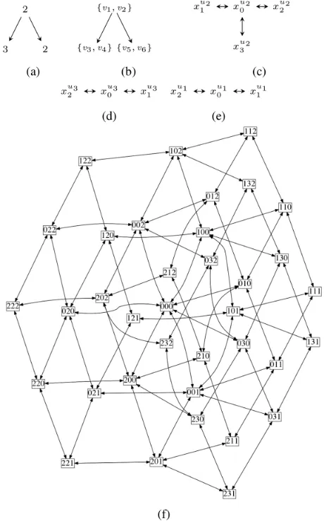
Figure 2: Referring to Example 6, (a) is a natural number labelled graph. (b) a lifted dependency graph of the factored systemδfrom Example 6. (c), (d), (e) are the largest con-nected components in the state spaces of the systems 4u2, 4u3
and4u1
, respectively. (f) is the largest connected compo-nent in the state space ofδ.
Example 6. This is an example of the construction from Theorem 3, for the natural number labelled digraphGNin
Figure 2a. InGNthere are three verticesu1(the root),u2,
andu3, labelled by the numbers 2, 3, and 2, respectively. We
construct three systems, one per vertex, shown in Figures 2c-2e. For u2 the constructed system is4
u2 = {(xu2
0 , x
u2
1 ),
(xu2
0 , x
u2
2 ),(x
u2
0 , x
u2
3 ),(x
u2
1 , x
u2
0 ),(x
u2
2 , x
u2
0 ), (x
u2
3 , x
u2
0 )}.
The states are defined asxu2
0 ={v3,v4},x1u2 = {v3,v4},
xu2
2 = {v3,v4},x3u2 = {v3,v4}. For u3 the constructed
system is 4u3 = {(xu3
0 , x
u3
1 ),(x
u3
0 , x
u3
2 ),(x
u3
1 , x
u3
0 ),(x
u3
2 ,
xu3
0 )}. The states are defined asx
u3
0 ={v5,v4},xu13 ={v5,
v4}and xu3
2 = {v5,v4}. Foru1 the constructed system is
4u1 ={(xu1
0 , x
u1
1 ),(x
u1
0 , x
u1
2 ),(x
u1
1 , x
u1
0 ),(x
u1
2 , x
u1
0 )}. The
states are defined asxu1
0 = {v1,v2},x1u1 ={v1,v2}, and
xu1
2 = {v1,v2}. For anyxui1, x u1
j ∈ S(4 u1),xu1
i x u1
j
holds and accordinglytd(4u1) = 2. Similarly,td(4u2) = 3 andtd(4u3) = 2.
The required witness isδ={(xu1
0 ]x
u2
0 , x
u2
1 ),(x
u1
0 ]x
u3
0 ,
xu3
1 )} ∪4
u1 ∪ 4u2 ∪
4u3, where the actions {(xu1
0 ]x
u2
0 ,
xu2
1 ),(x
u1
0 ]x
u3
0 , x
u3
1 )} add toδ dependencies equivalent
to the edges of GN, i.e. the dependencies shown in Fig-ure 2b. Also, in the constructed witness, for all states x0,
x1 ∈ S(δ)(shown in Figure 2f)x0 x1 holds, and
ac-cordinglytd(δ) = 35.
Computing the Traversal Diameter
An important aspect oftdis that, unlike the diameter or the recurrence diameter, it can be computed in linear time us-ing Algorithm 1. A principal component of computus-ing the traversal diameter is an algorithm to compute the weight of the “weightiest” path in acyclic digraphs, where vertices are assigned numerical weights. The weight of a path is the sum of weights of all the vertices that it traverses added to the number of edges comprising it. The weightiest path is com-puted using the recurrenceSmax.
Definition 12 (Weighted Longest Path). For a digraphG, let the functionb: V(G)⇒ Nbe a function that assigns a
natural number for every vertex inV(G).Sis
Shbi(u,G) =b(u) + max
u0∈childG(u)(Shbi(u
0,G) + 1)
Then, letSmaxhbi(G) = max
u∈V(G)Shbi(u,G).
Smax is only well-defined if G is acyclic. The runtime of Smaxis linear in the size ofV(G), if the values ofSfor dif-ferent vertices are memoised and assuming thatbis at most of linear complexity. Accordingly if we use Tarjan’s (Tarjan 1972) algorithm to compute the strongly connected compo-nents, the runtime of Algorithm 1 would be linear in the size of the state space of the given system.
Algorithm 1:TRAVD(δ)
SCC:= set of strongly connected components ofG(δ) returnSmaxhCi(G(δ)/SCC), whereC(s) =|s| −1
Theorem 4. TRAVD(δ) =td(δ).
andchild(scc) =childG(scc). SinceGis a DAG, its vertices
can be topologically ordered in a listlSCC.
Firstly, we prove TRAVD(δ) ≤ td(δ). We show that for any strongly connected componentscc ∈ Gthere is an ac-tion sequence→πscc ∈δ∗and a statexscc ∈ scc, such that
S(scc)≤ |ss(xscc,
→
πscc)| −1, which from Definitions 11
and 12, implies TRAVD(δ) ≤ td(δ). We prove this by in-duction onlSCC. The base case,lSCC = [], is
straightfor-ward. For the step caselSCC =scc :: l0SCC,1 and for any
scc0 ∈ l0SCC, there is a state x0 ∈ scc0 and an action se-quence→π0 ∈ δ∗ whereS(scc0) ≤ |ss(x0,→π0)| −1. Since sccis a strongly connected component of states inG(δ), then
there is→π0scc ∈δ∗ and a statexscc ∈scc, where
→
πscc
tra-verses exactly all the states inscc, if executed atxscc∈scc,
i.e.ss(xscc,
→
π0scc) =scc. We have two cases:
Case 1 (child(scc) = ∅). From Definition 12, S(scc) =
|scc| −1 =|ss(xscc,
→
π0scc)| −1holds for this case. Accord-ingly the required witness→πsccis the same as
→
π0scc.
Case 2 (child(scc) 6= ∅). Let sccmax be a strongly
con-nected component where∀ scc0 ∈ child(scc). S(scc0) ≤
S(sccmax). Becausesccmax∈child(scc)we havesccmax∈
lSCC0 , and accordingly from the inductive hypothesis there arexmax ∈sccmaxand
→
πmax ∈ δ∗ such thatS(sccmax)≤
|ss(xmax,
→
πmax)| −1.(†) Also, becausesccmax∈child(scc)
and since bothsccandsccmaxare strongly connected
com-ponents, there must be→π0 ∈ δ∗, where→π0scc_→π0(xscc) =
xmax. 2 We now show that →πscc =
→
π0scc_→π0_→πmax is the required witness. First, it is easy to see that
ss(xscc,
→
π0scc)∪ss(xmax,
→
πmax) ⊆ ss(xscc,
→
πscc). Since
sccmax ∈ child(scc), thenss(xmax,
→
πmax)is disjoint with
scc. Accordingly |ss(xscc,
→
π0scc)| + |ss(xmax,
→
πmax)| ≤
|ss(xscc,
→
πscc)|. From this, (†), and Definition 12 we have
S(scc)≤ |ss(xscc,
→
πscc)| −1.
Secondly, we provetd(δ)≤TRAVD(δ)by showing that for any scc ∈ G, xscc ∈ scc, and
→
πscc ∈ δ∗, we have
|ss(xscc,
→
πscc)| −1 ≤ S(scc). Our proof is again by
in-duction on the list lSCC. The base case, lSCC = [], is
straightforward. The step case lSCC = scc :: lSCC0 , and
we have that for anyscc0 ∈l0
SCC,x0 ∈scc0, and
→
π0 ∈δ∗,
|ss(x0,→π0)| −1≤S(scc0)holds. We have two cases:
Case 1(ss(xscc,
→
πscc)⊆scc). Sincess(xscc,
→
πscc)⊆scc
then |ss(xscc,
→
π)| ≤ |scc|. From Definition 12, we know that|scc| −1≤S(scc), and accordingly|ss(xscc,
→
πscc)| −
1≤S(scc).
Case 2 (ss(xscc,
→
πscc) 6⊆ scc). Since ss(xscc,
→
πscc) 6⊆
scc, then there are →πscc, π, and
→
πchild such that:
1
For a listl,h::lislwith the elementhappended to its front.
2
For two listsl1andl2,l1_l2denotes their concatenation.
(i) →πscc =
→
π0scc_π ::
→
πchild, (ii) ss(xscc,
→
π0scc) ⊆ scc,
and (iii) letting xchild = π(
→
π0scc(xscc)), xchild ∈ sccchild
holds, for somesccchild∈child(scc). Using the same
argu-ment as the last case, we have|ss(xscc,
→
π0scc)| ≤ |scc|.(*)
Since xchild ∈ sccchild, and from the inductive hypothesis,
we have that|ss(xchild,
→
πchild)| −1≤S(sccchild). Then
us-ing (*) and sincess(xchild,
→
πchild)andsccare disjoint, we
have|ss(xscc,
→
πscc)| −1≤ |scc|+S(sccchild). From
Defi-nition 12, we have|scc|+S(sccchild)≤S(scc)and accord-ingly|ss(xscc,
→
πscc)| −1≤S(scc).
Example 7. Consider the projection δvs1 of δ from Example 2 as input to Algorithm 1. The first step in Algorithm 1 is to compute the SCCs of the state space G(δ). G(δ) is shown in Figure 1b, and it has three strongly connected components, thus SCC :=
{{v1v2,v1v2},{v1v2},{v1v2}}. Those connected
compo-nents induce the quotient of the state space shown in Fig-ure 1f. Next, the algorithm computesSmaxhCi(G(δ)/SCC). We have ShCi({v1v2}) = C({v1v2}) = 0, and
ShCi({v1v2}) = C({v1v2}) = 0.ShCi({v1v2,v1v2}) = C{v1v2,v1v2}+max{ShCi({v1v2}),ShCi({v1v2})}+1 =
1+0+1 = 2. Thus,SmaxhCi(G(δ)/SCC) = 2, which is the
traversal diameter of the state space ofδvs
1and the value returned by Algorithm 1.
Tightness of the Traversal Diameter
Having a product of the traversal diameters of all projections as a compositional bound may not seem like a practically helpful bound. However, it is a substantial improvement over what can currently be done in the case when there is not a non-trivial acyclic lifted dependency graph. When given a set of projections without acyclicity in the dependencies between them, existing compositional bounding approaches use the product of the projected state space sizes EXP(δ)as a bound (Rintanen and Gretton 2013, AGN1, and AGN2). Using the product bound of Theorem 2 is a substantial im-provement over that because, as shown in the next theorem, the traversal diameter can be exponentially smaller than the size of state space.
Theorem 5. There are infinitely many factored systems whose traversal diameters are exponentially smaller (in the number of state variables) than the size of their state spaces.
Proof. For an arbitrary numbern∈N, we construct a sys-tem whose state space size is a factor of n more than its traversal diameter. Letxi, for0 ≤i ≤ n, ben+ 1states.
Consider the system{(x0, xi)| 1 ≤i ≤n}. The traversal
diameter of this system is1since, the only possible transi-tions are from statex0to a statexi, for1≤i≤n. However
the system’s state space has at leastn+ 1states.
Example 8. δvs
2 from Example 2 whose state space is shown in Figure 1c is an example of the above construction withn= 3. We can takex0, x1, x2, andx3to bev3v4,v3v4,
Practical Bounding Using the Traversal
Diameter
In the last section, we laid down a theoretical foundation suggesting that the traversal diameter could be successfully used for compositional upper bounding. A schema for algo-rithms utilising that theoretical framework to composition-ally bound the traversal diameter of a systemδis
ARB(δ) = ch
vs1..n∈VS1..n
Π
vs∈vs1..n(TRAVD(δvs) + 1)−1
Above,VS1..n denotes the set of all partitions of the set of
state variablesD(δ), andchdenotes a function that chooses one partitionvs1..nto use for compositional bounding.
To fully specify the bounding algorithm ARBwe need to determine the choice of the partition of D(δ)using which we obtain the projections. Optimally, the functionchwould be instantiated with the function min that would choose the partition which results in the smallest bound. However, since the size ofVS1..nis intractable,minwould be an
im-practical solution. We adopt a im-practically feasible approach used by AGN2: we take the situation whereD(δ) models all assignments in the SAS+ model generated using Fast-Downward’s preprocessing step (Helmert 2006), and choose
chto return a partitionvs1..n s.t. each equivalence class in
vs1..nhas elements that model all the assignments of exactly
one SAS+ state variable.
Now that we have fully specified ARBwe compare it to other bounding algorithms. We experimentally evaluate dif-ferent bounding algorithms on problems from previous In-ternational Planning Competitions (IPC), and the unsolv-ablity IPC, open Qualitative Preference Rovers benchmarks from IPC2006 (to which we refer as NEWOPEN) and the hotel-key protocol verification problem from AGN2. Our ex-periments were conducted on a uniform cluster with time and memory limits of 30minutes and 8GB, respectively.
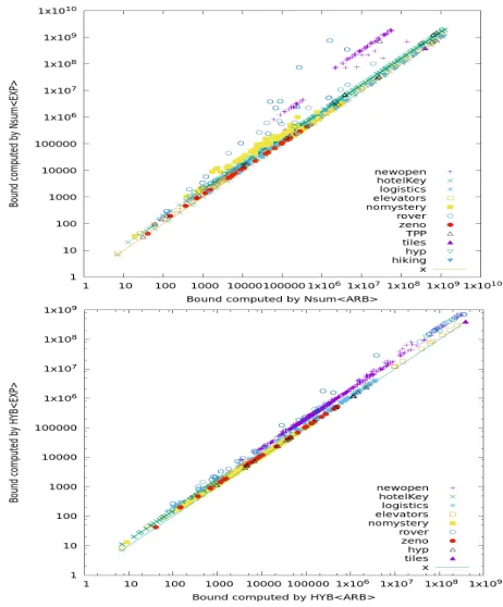
The first two columns in Table 1 show that compared to
NsumhEXPi, ARBfails to compute bounds tighter than109
in most domains. That is because when there is branching in the dependency graph,Nsum computes a bound that has additive terms like the ones in Example 4, while on the other hand, ARBalways returns a bound that is the product of the projections’ traversal diameters.
Now, recall that Theorem 5 predicts the possibility for ex-ponential improvement in the computed bound if, instead of EXP, we use ARBto bound a system. This suggests an-other utilisation of ARB: to use it as a base case function forNsuminstead of EXP. This way ARBwill be only used
to bound projections which cannot be further decomposed byNsum, i.e. projections whose variable dependencies are
strongly connected. Indeed, using ARBas a base case func-tion improves the computed bounds in 71% of the problems, and the improvement is at least 50% in 66% of the cases. The second row in Table 1 gives an overview of the improve-ment in the bounds computed byNsumhARBicompared to NsumhEXPifor different domains. A more detailed compar-ison is in the top plot of Figure 3.
The Traversal Diameter and State Space
Acyclicity
The construction used in the proof of Theorem 3 suggests that the bounds computed by ARBare better than those com-puted by EXP only if the projections of the system have acyclicity and “branching” in their state space. In fact the following proposition holds.
Proposition 4. IfG(δ)is strongly connected, thentd(δ) =
EXP(δ).
This begs the question of whether ARB can somehow be combined with the algorithm proposed by AGN2, which also exploits acyclicity in the state space, to compute tighter bounds and better system decompositions. We first review the approach of AGN2. A critical element of their approach is a system abstraction to which they refer as asnapshot. It models the system when we fix the assignment of a subset of the state variables, removing actions whose preconditions oreffects contradict that assignment.
Definition 13 (Snapshot). For states x and x0, let
agree(x, x0)denote|D(x)∩ D(x0)| = |x∩x0|, i.e. every variable that is in the domains of bothxandx0has the same assignment inxandx0. The snapshot ofδat a statexis
δ|•x={(p, e)|(p, e)∈δ∧agree(p, x)∧agree(e, x)}D(x)
whereD(x)denotesD(δ)\ D(x).
Based on snapshots, and given a systemδ, a set of vari-ablesvs, and a base case functionb, AGN2 defined a method
Smaxhbi(vs, δ).3That method computes the weightiest path
in the state spaceG(δvs), where the weight of a statexis b(δ•|x). It is only defined ifG(δvs)is acyclic. Combining
Smax andNsum, AGN2 suggested Algorithm 2 as a hybrid
approach to exploit acyclicities in state spaces and depen-dencies. In HYB,vs1..nis a partition ofD(δ), andac(vs1..n)
is a member of vs1..n s.t. the projectionδac(vs1..n)has a
non-trivial acyclic state space. HYBinterleaves the functions
NsumandSmax. It only callsSmaxif the given system’s
de-pendencies are strongly connected andδhas acyclic projec-tions on members ofvs1..n. If bothNsum andSmaxcannot
be called, HYBuses EXPas a base case function.
Algorithm 2:HYB(δ,vs1..n)
SCC :=set of strongly connected components ofGD(δ) GVS:=GD(δ)/SCC
if2≤ |V(GVS)|
returnNsumhHYB(•,vs1..n)i(δ,GVS)
if∃vsi=ac(vs1..n)
vsi:=ac(vs1..n)
returnSmaxhHYB(•,vs1..n\ {vsi})i(vsi, δ)
returnEXP(δ)
Example 9. From Examples 1 and 2, consider the system δ and the partition vs1..n = {vs1,vs2} of its state
vari-ables. The SCCs of the dependency graph of δ are vs1
3
and vs2, and thus the lifted dependency graphGVS
com-puted by HYB is the one in Example 3. Accordingly, HYB
will return NsumhHYB(•,vs1..n)i(δ,GVS). Then we have
that NsumhHYB(•,vs1..n)i(δ,GVS) = HYB1 + HYB2 +
HYB1HYB2, where HYBi = HYB(δvsi,vs1..n) for i ∈
{1,2}. Sinceδvs2has the acyclic state space shown in Fig-ure 1c we haveHYB2 =SmaxhHYB(•,vs1)i(vs2, δvs2) = 1. Since the state space of δvs1 is not acyclic, HYB1 = EXP(δvs1) = 3. Thus,HYB(δ,vs1..n) = 1 + 3 + 1×3 = 7.
Since HYB already exploits state space acyclicity using
Smax, the main question now is whether using ARB as a base case function for HYBinstead of EXPcan improve the computed bounds. The short answer to that question is: yes, bounds computed by HYBusing ARBas a base case func-tion are better in 68% of the problems compared to those computed with EXPas a base case, and the improvement is at least 50% in 71% of the cases. The third column of Ta-ble 1 and the bottom plot of Figure 3 show a fine-grained comparison between the bounds.
To understand the improvement in the computed bounds, recall that if the dependency graph has one SCC, HYBwill pick one vsi from vs1..n, s.t. the state space of δvsi is
acyclic. Then HYB usesSmax to decompose δinto
multi-ple abstractions: the projectionδvsi and the snapshots ofδ on the different states inU(δ). ThenSmaxcalls HYB recur-sively on each of the snapshots ofδ, withvsiremoved from
vs1..n. This is repeated until the state space of the projection
on each remaining member ofvs1..n is not acyclic. Then
the base case function is called to bound the projection on
Figure 3: Top (resp. bot.): bounds computed byNsum(resp.
HYB) when EXP(vert.) is base case function vs ARB(hor.).
Table 1: Col. 1: the domain name and the number of prob-lems in it. Col. 2: the number of probprob-lems for which ARB computed a bound less than 109. Col. 3 (resp. 4) has
four numbers: (i) problems for which NsumhEXPi (resp. HYBhEXPi) computed a bound less than 109 (ii)
prob-lems for which NsumhARBi (resp. HYBhARBi) computed
a bound less than 109 (iii) problems for which the bound
byNsumhARBi(resp. HYBhARBi) is less than the bound by NsumhEXPi(resp. HYBhEXPi) (iv) problems for which the bound byNsumhARBi (resp. HYBhARBi) is less than half
the bound byNsumhEXPi(resp. HYBhEXPi).
the remaining members ofvs1..n. However, as shown in the
next example, if a projection’s state space is not acyclic, its traversal diameter can still be much tighter than the size of its state space. This will lead to much tighter bounds com-puted by HYBif it uses ARBas a base case function instead of EXP.
Example 10. Consider the computation in Example 9. If ARB is used as a base case function, HYB1 =
ARB(δvs1,vs1..n) = TRAVD(δvs1) = 2 (for the evaluation of TRAVD(δvs1) see Example 7). Thus HYB(δ,vs1..n) = 1 + 2 + 1×2 = 5.
un-satisfiable planning problems that other state-of-the-art plan-ners could not solve. We now study the improvement in the coverage of MPif we use as horizons the bounds computed by HYB when ARB is the base case. Compared to using EXPas a base case, ARBincreases the coverage by 234 for solvable problems. Those problems come from the domains: NEWOPEN (221 problems), ROVER (7 problems), SATEL -LITE(5 problems), and TPP (1 problem). Also, using ARB as a base case for HYBallows MPto prove the unsolvability of an additional 4 problems from the domainNEWOPENand 52 problems from the domain HOTELKEY, that it could not solve when EXPis used as a base case function.
Conclusions and Future Work
We contributed a novel compositional upper bounding ap-proach in planning. Our technique exposes problems with a relatively wide variety of dependency structures to upper bounding. Previous approaches only apply to a limited class of problems that have a branching 1-way state variable de-pendency structure. Our analysis treats a much broader class of problems, with 2-way dependencies. Our new approach, however, is most useful when combined with other existing compositional bounding techniques, where it leads to sub-stantial improvement in the computed bounds. We use it to decompose problem abstractions produced using the other compositional bounding techniques when those abstractions have bidirectional dependencies.
An open problem is to devise a method to practically de-compose large concrete problems with strongly connected dependencies instead of only small abstractions produced by other compositional algorithms. Also, investigating the ef-fect of the partition of the state variables used to decompose problems on the value of computed bounds is an interesting avenue for future research.
Acknowledgements We thank Dr. Charles Gretton, Dr. Michael Norrish, Lars Hupel and Simon Wimmer for proof-reading parts of this paper, and Lars Hupel for helping me set up the experiments. We also thank Prof. Tobias Nipkow and the German Research Foundation for funding that facilitated this work through the DFG Koselleck Grant NI 491/16-1.
References
Abboud, A.; Williams, V. V.; and Wang, J. 2016. Approx-imation and fixed parameter subquadratic algorithms for ra-dius and diameter in sparse graphs. InProceedings of the twenty-seventh annual ACM-SIAM symposium on Discrete Algorithms, 377–391. SIAM.
Abdulaziz, M.; Gretton, C.; and Norrish, M. 2015. Veri-fied Over-Approximation of the Diameter of Propositionally Factored Transition Systems. InInteractive Theorem Prov-ing. Springer. 1–16.
Abdulaziz, M.; Gretton, C.; and Norrish, M. 2017. A State Space Acyclicity Property for Exponentially Tighter Plan Length Bounds. InInternational Conference on Automated Planning and Scheduling (ICAPS). AAAI.
Abdulaziz, M. 2017. Formally Verified Compositional Al-gorithms for Factored Transition Systems. The Australian National University.
Aingworth, D.; Chekuri, C.; Indyk, P.; and Motwani, R. 1999. Fast estimation of diameter and shortest paths (with-out matrix multiplication). SIAM Journal on Computing 28(4):1167–1181.
Alon, N.; Galil, Z.; and Margalit, O. 1997. On the exponent of the all pairs shortest path problem. Journal of Computer and System Sciences54(2):255–262.
Baumgartner, J.; Kuehlmann, A.; and Abraham, J. 2002. Property checking via structural analysis. In Computer Aided Verification, 151–165. Springer.
Biere, A.; Cimatti, A.; Clarke, E. M.; and Zhu, Y. 1999. Symbolic model checking without BDDs. InTACAS, 193– 207.
Chan, T. M. 2010. More algorithms for all-pairs short-est paths in weighted graphs. SIAM Journal on Computing 39(5):2075–2089.
Chechik, S.; Larkin, D. H.; Roditty, L.; Schoenebeck, G.; Tarjan, R. E.; and Williams, V. V. 2014. Better approxi-mation algorithms for the graph diameter. InProceedings of the Twenty-Fifth Annual ACM-SIAM Symposium on Discrete Algorithms, 1041–1052. Society for Industrial and Applied Mathematics.
Fredman, M. L. 1976. New bounds on the complexity of the shortest path problem. SIAM Journal on Computing 5(1):83–89.
Helmert, M. 2006. The Fast Downward planning system. Journal of Artificial Intelligence Research26:191–246. Kautz, H. A., and Selman, B. 1992. Planning as satisfiabil-ity. InECAI, 359–363.
Knoblock, C. A. 1994. Automatically generating abstrac-tions for planning. Artificial Intelligence68(2):243–302. Pardalos, P. M., and Migdalas, A. 2004. A note on the com-plexity of longest path problems related to graph coloring. Applied Mathematics Letters17(1):13–15.
Rintanen, J., and Gretton, C. O. 2013. Computing upper bounds on lengths of transition sequences. InInternational Joint Conference on Artificial Intelligence.
Rintanen, J. 2012. Planning as satisfiability: Heuristics. Ar-tificial Intelligence193:45–86.
Roditty, L., and Vassilevska Williams, V. 2013. Fast ap-proximation algorithms for the diameter and radius of sparse graphs. InProceedings of the Forty-Fifth Annual ACM Sym-posium on Theory of Computing, 515–524. ACM.
Tarjan, R. 1972. Depth-first search and linear graph algo-rithms. SIAM Journal on Computing1(2):146–160. Williams, B. C., and Nayak, P. P. 1997. A reactive planner for a model-based executive. InInternational Joint Confer-ence on Artificial IntelligConfer-ence, 1178–1185. Morgan Kauf-mann Publishers.