25
Modern robust statistical methods can provide substantially
higher power and a deeper understanding of data
Rand R. Wilcox
Department of Psychology, University of Southern California, 3620 McClintock Ave, Los Angeles, CA 90089-1061, USA
Received May 1, 2014: Revised May 30, 2014: Accepted June 5, 2014: Published online June 30, 2014
Abstract
During the last fifty years, there have been many advances and insights relevant to the most basic statistical methods, designed to compare groups and study associations. Classic, routinely used methods assume sampling is from a normal distribution. Numerous papers make it clear that violating this assumption can result in missing true differences among groups and true associations among variables. Many new methods have been derived that are designed to perform well when dealing non-normal distributions and outliers that can make a substantial difference when analyzing data. Broadly, modern technology offers the opportunity to get a deeper and more accurate understanding of data. The paper reviews the basic reasons why standard methods can be highly unsatisfactory and provides an overview of some of the more modern methods that have been derived. Comments on SPSS and the software R are included.
Key words : Robust statistical methods, outliers, SPSS, software R
1. Introduction
Robust statistical methods capable of dealing with large complex data sets, are required more than ever before in almost all branches of science. Robust statistical methods offer the opportunity to substantially improve the reliability and accuracy of statistical modeling and data analysis. It is ideal for researchers, practitioners and graduate students of statistics, electrical, ch emical and biochemical engineering, and computer vision. There is also much to benefit researchers from other sciences, such as biotechnology and life sciences. Outliers often indicate the most interesting data point, like polluted areas for environmental data, or irregularities in online monitoring of patients. Among many such applications are: monitoring and tracking the condition of patients in intensive care
via several measurements such as pulse rate, blood pressure, lung water etc. Without robust analysis methods, it is easy to miss significant outliers in such multivariate data.In some cases, the outliers only show up clearly when considering all the variables together, and yet may indicate something significant that could easily be missed, such as a sudden deterioration in a critical patient’s condition.
In pharmaceutical manufacturing processes, time oriented quality characteristics, such as the degradation of a drug, are often of interest. Robust methods can be applied to pharmaceutical production research an d developmen t by proposin g experimen tal an d
Author for correspondence: Professor Rand R. Wilcox
Department of Psychology, University of Southern California, 3620 McClintock Ave, Los Angeles, CA 90089-1061, USA
E-mail: [email protected] Tel.: +91-(213) 740–2258
Copyright @ 2014 Ukaaz Public ations. All rights reserved. Email: [email protected] om; Website: www.ukaazpublications.com
optimization models, which should be able to handle the time-oriented characteristics. In the pharmaceutical industry, the development of a new drug is a lengthy process, involving laboratory experiments. When a new drug is discovered, it is important to design an appropriate pharmaceutical dosage or formulation for the drug so that it can be delivered efficiently to the site of action in the body for the optimal therapeutic effect on the intended patient population. Hence, the quality of the pharmaceutical product is influenced by such design when they are applied in the early stages of drug development. Modern robust statistical methods can play vital role toward this goal (Cho and Shin, 2012).
It was once thought that routinely used statistical methods for comparing groups and studying associations perform reasonably well when dealing with non-normal distributions. But modern insights have revealed that under general conditions, classic methods can miss important differences among groups and important associations among two or more variables. In more technical terms, standard techniques can have relatively poor power compared to more modern methods. Moreover, standard techniques can miss features of the data that have considerable practical importance (e.g., Heritier et al., 2007; Huber and Ronchetti, 2009;Marrona
et al., 2006; Rousseeuw and Leroy, 1987; Staudte and Sheather, 1990; Wilcox, 2012a,b). A positive feature of routinely used methods is that they are robust to violations of assumptions when comparing groups that do not differ in any manner (they have identical distributions). When studying associations, conventional methods perform well when there is no association.More precisely, they control the probability of a Type I error reasonably well. If groups differ or there is an association, of course classic techniques might continue to perform well, but under general conditions this is not the case, even when the sample sizes are large.More broadly, complete reliance on routinely used methods can result in a relatively superficial and misleading understanding of data. This has serious
PHYTOMEDICINE An International Journal
Annals of Phytomedicine 3(1): 25-30, 2014 Journal homepage: www.ukaazpublications.com
implications regarding the choice of software: SPSS is commonly used but it is poorly equipped to take advantage of modern technology. Easily the best software for taking advantage of modern methods is the software R.
A detailed description of the many improved statistical techniques that have practical value is impossible in a single paper. The goal in this review is to describe some aspects of modern methods in the hope of increasing awareness of these advances and improving future studies.
1.1 Limitations of classical statistical methods
Appreciating the practical importance of modern robust methods requires in part some understanding of when and why more conventional methods,based on means and least squares regression, can be unsatisfactory. There are a variety of concerns associated with standard methods, many of which center around three major insights.
2. Detecting outliers
Before describing the three major insights just mentioned,it helps to first comment briefly on methods aimed at detecting outliers. A common approach is to declare a value an outlier if it is more than two or three standard deviations from the mean. But this method is well known to be unsatisfactory, roughly because outliers can inflate the standard deviation, which results in outliers being masked (e.g., Rousseeuw and Leroy, 1987; Wilcox, 2012a). The general strategy for dealing with this problem is to replace the mean and standard deviation with measures of location (measures of central tendency) and scale (measures of variation) that are relatively insensitive to outliers. Two such methods are the boxplot and the so-called MAD -median rule. From basic principles, the boxplot is based on the interquartile range, meaning that more than 25% of the values would need to be outliers for it to break down.
As for the MAD-median rule, consider n observations: X1, . . . , Xn, let M be the usual sample median and let MAD indicate the median absolute deviation statistic, which is the median based on
|X1 – M |, . . . , |Xn – M |. Then the MAD median rule declares Xiand
outlier if
where MADN is MAD/.6745. (Under normality, MADN estimates the standard deviation.) The MAD-median rule can accommodate more outliers than the boxplot without breaking down. The relative merits of these two outlier detection methods are discussed in more detail in (Wilcox, 2012b).
It is noted that when dealing with multivariate data, a seemingly natural strategy is to simply use the MAD-median rule on the each of the variables. A concern, however, is that this does not take into account the overall structure of the data. For example, it is not unusual for someone to be young, it is not unusual for someone to have heart disease, but it is unusual to be both young and have heart disease. Methods for dealing with multivariate data have been derived (e.g., Wilcox, 2012b), but the details go beyond the scope of this review.
3. Three major insights
The first major insight has to do with how large of a sample is needed in order to assume normality. Consider the one-sample Student’s t test. At one time, it was thought that with a sample size of about 30, normality can be assumed. This was a natural conclusion based on early studies indicating that with a relatively small sample size, the sample mean has, to a good approximation, a normal distribution under fairly weak conditions. But more recent studies clearly indicate that even when the sample mean has a roughly normal distribution, Student’s t can perform poorly in terms of controlling the Type I error probability (rejecting a true hypothesis).
As an illustration, consider a skewed distribution for which the proportion of points declaredan outlier will be relatively small based on a boxplot or the MAD-median rule. Suppose that a nominal .05 Type I error probability is judged to be reasonably accurate if the actual Type I probability is between .025 and .075. Then approximately 200 observations are required when using Student’s t. When dealing with a skewed distribution where outliers are relatively common, now 300 observations can be required (e.g., Wilcox, 2012b). This has implications regarding the two-sample t test. If the two distributions under study have different amounts of skewness, Student’s t might yield relatively inaccurate confidence as illustrated in Wilcox (2012a). In fact, Cressie and Whitford (1986) describe general conditions where the two-sample t test is inaccurate regardless of how large the sample sizes might be.
The second insight has to do with the extreme sensitivity of the population variance to the tails of a distribution, which has serious negative implications about power, the probability of rejecting the null hypothesis when it is false. Even arbitrarily small changes in a distribution, in a sense made precise, for example, in Staudte and Sheather (1990) and Wilcox (2012b), can substantially impact the population variance, which in turn can result in relatively low power when testing hypotheses based on the sample mean.
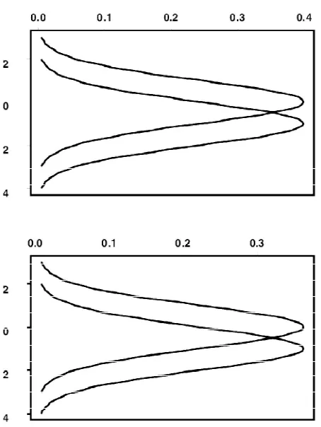
A classic example is shown in Figure 1. The left panel shows two normal distributions, both of which have variances equal to one. With both sample sizes equal to 25, power is .96 when testing at the .05 level with Student’s t. Now look at the right panel, which shows two distributions that have thicker tails than the normal distribution. Now power is only .28 despite the apparent similarity with the normal distributions in the left panel. The reason is that these distributions are not normal, they are mixed normals that have variance 10.9. (The mixed normal used here means that with probability .9, an observation is randomly sampled from a standard normal distribution, otherwise an observation is sampled from a normal distribution having mean zero and standard deviation 10.)This illustrates the general principle that inferential methods based on means are highly sensitive to the tails of the distributions, roughly because even small changes in the tails of a distribution can have an inordinate influence on the variance.
Figure 1:In the left panel, power is .96 based on Student’s t, = .05 and sample sizes n
1= n2= 25. But in the right panel, the distributions are not normal and power is only .28
4.
Regression and Pearson’s Correlation
Pearson’s correlation and conventional (least squares) regression techniques suffer from the same problems associated with methods based on means and new concerns arise. Even a single outlier has the potential of distorting the nature of the association among the bulk of the participants. When there is heteroscedasticity (the variance of the dependent variable depends on the value of the independent variable), conventional confidence intervals use the wrong standard error, which in turn can mean inaccurate confidence intervals regardless of how large the sample size might be. Another concern is that relationships between variables can be more complex and poorly modeled by the more obvious parametric models such as a straight line or a quadratic fit.
5. Some unsatisfactory strategies for dealing with
normality and outliers
Simple transformations are sometimes suggested for salvaging methods based on means, such as taking logs.But by modern standards this approach is unsatisfactory: typically distributions remained skewed and the deleterious impact of outliers remains (e.g., Rasmussen, 1989; Doksum and Wong, 1983; Wilcox and Keselman, 2003).
A seemingly natural way of dealing with outliers is to remove them and apply some method for means to the remaining data. This is reasonable provided a compelling argumentcan be made that the outliers are invalid. But otherwise, this can result in highly inaccurate
conclusions regardless of the sample sizes (Bakker and Wicherts, in press; Wilcox, 2012a,b). There are technically sound methods for dealing with outliers, some of which are illustrated here, but they are not remotely obvious based on standard training. Another way of trying to salvage classic methods is to test the assumptions of normality and homoscedasticity. For example, test for equality of variances, if the result is not significant, use the pooled variance Student’s t-test and if the result is significant, use Welch’s test. However, all indications are that this strategy performs poorly (e.g., Hayes and Cai, 2007; Markowski and Markowski, 1990; Moser, Stevens and Watts, 1989; Wilcox, Charlin and Thompson, 1986; Zimmerman, 2004). A similar result was reported by Ng and Wilcox (2011) when dealing with least squares regression.The basic problem is that unless the sample size is sufficiently large, assumption tests frequently fail to detect violations of assumptions that are a practical concern.Presumably with a sufficiently large sample size, testing assumptions is satisfactory, but it remains unclear when this is the case.
Figure 2: Plots of means and medians when sampling from a normal, heavy-tailed and skewed distributions
with greater accuracy than the population mean. This has practical importance because Tukey (1960) predicted that we should expect outliers in practice and modern outlier detection methods confirm that outliers are routinely encountered.
Next, consider a skewed (lognormal) distribution. The right portion of Figure 2 shows boxplots of the resulting means and medians.This illustrates that even when a skewed distribution has relatively light tails (meaning that the expected proportion of values that are outliers is relatively small), it can be difficult getting an accurate estimate of the population mean compared to other measures of central tendency.
6. Nonparametric (rank-based) tests
Switching to classical nonparametric statistical tests for detecting group differences, such as the Wilcoxon-Mann-Whitney (WMW) U test or the Friedman test, is another approach to dealing with non-normal data. Rank based methods provide information that differs from methods based on measures of central tendency, as they are sensitive to different features of the distributions under study. The WMW test, for example, is sometimes suggested as a method for comparing medians, but generally it does not address this goal (e.g., Hettmansperger, 1984; Fung, 1980). Let p be the probability that a randomly sampled observation from the first group is less than a randomly sampled observation from the second. The WMW test is based on an estimate of p, but it does not provide a satisfactory test of p=.5 or an accurate confidence interval for p, roughly because it uses the wrong standard error when distributions differ (cf. Zimmerman, 1998, 2000). That is, the derivation of the standard error assumes that the two groups have identical distributions. So in effect, when significant results are found using the WMW, it is reasonable to conclude that the distributions differ, but the details regarding how they differ and by how much are unclear (To get accurate confidence intervals for p, see Cliff, 1996; Brunner and Munzel, 2000; Wilcox, 2012a, b.)
7. Modern robust methods
There is a vast literature aimed at dealing with the limitations of classical statistical methods (e.g., Hampel, et al. 1986; Heritier et al., 2009; Huber and Ronchetti, 2009; Marrona et al., 2006; Rousseeuw and Leroy, 1987; Staudte and Sheather, 1990; Wilcox, 2012a, b). The problem is not finding a method that deals with skewed distributions, outliers and heteroscedasticity in a relatively effective manner. Many such methods are available. Moreover, these new techniques provide different perspectives that help deepen our understanding of data. This is particularly true when dealing with regression and correlation (e.g., Wilcox, 2012b, ch. 10-11). The details of the many improved methods for comparing groups and studying associations cannot be described in a single paper. Instead, their more basic features are briefly described and illustrated.
7.1 Comparing means
It is possible to improve the accuracy of hypothesis tests and confidence intervals for means by using a computer intensive method called bootstrapping. These newer techniques have considerable practical value (Wilcox, 2012a, b), but when using means, inaccurate confidence intervals can still result with a sample size of 100 when distributions are skewed and outliers are common (Hayes and Cai, 2007; Wilcox, 2012a, p. 273). Moreover, even for symmetric
distributions, methods based on means can result in relatively poor power.In order to fully deal with these problems, it is necessary to switch to some measure of central tendency other than the mean.
7.2 Comparing medians
A seemingly obvious way of dealing with skewness and outliers is to use the median. However, most hypothesis testing methods for comparing medians can be very inaccurate when there are tied (duplicated) values, or when there is heteroscedasticity (e.g., Wilcox, 2012a, b). A solution is to use a slight generalization of another basic bootstrap method, called a percentile bootstrap method, which is able to effectively deal with both of these problems, even for small sample sizes, such as 10 per group (Wilcox, 2006). A positive feature of comparing groups using medians is that, in terms of hypothesis testing, power can be high relative to other methods that might be used when outliers are common.
7.3 Comparing trimmed means
Trimmed means contain the mean and median as special cases. The mean reflects no trimming and the median is based on the maximum amount of trimming. A trimmed mean is computed by removing a certain percentage of the highest and lowest values and then averaging the remaining scores. For example, to compute a 20% trimmed mean, the scores are ordered from smallest to largest, the lowest and highest 20% are removed,and the mean of the remaining scores is calculated. Trimming can be an effective strategy for handling skewed and heavy tailed distributions because it eliminates outliers and it results in more accurate confidence intervals compared to conventional methods based on the mean.
It is stressed that simply trimming the extreme values and then using classical methods for means, such as a t-test in SPSS, is technically unsound and yields highly inaccurate results even when the sample size is large (Briefly, the standard error is not being estimated correctly). Technically sound methods are available as well as appropriate software (Wilcox,2012a, b) but no details are given here.
An important consideration when comparing groups using trimmed means is how much to trim, as different amounts of trimming can yield different conclusions. Trimming too little can result in inaccurate confidence intervals, but trimming too much can result in unnecessarily wide confidence intervals and low power when testing hypotheses. As a general guideline, using 20% trimming is a good compromise for general use. But is suggested that in exploratory studies, multiple perspectives can be very useful.
8. Correlation and Regression
Skipped correlations make up a class of correlation coefficients that are of particular interest as they can deal with outliers that can negatively impact other coefficients. Roughly, they eliminate outliers using a multivariate outlier detection technique that takes into account the overall structure of the data and then they apply Pearson’s correlation, or even Spearman’s rho or Kendall’s tau, to the remaining data. One version that seems to perform relatively well is the so-called OP (outlier projection) correlation; see, for example Wilcox (2012b, section 15.5.5).
9. Software
SPSS is popular among academics, but it is poorly equipped to take advantage of modern statistical methods and it has become increasingly expensive. The result is that the number of academics using SPSS has declined substantially in recent years. Easily the best software for applying modern methods is the free software R(R Development Core Team, 2013), which can be downloaded from www.r-project.org/. Numerous books now describe how to use R and it now dominates how most statisticians analyze data. Users familiar with SAS and SPSS might find the book by Muenchen (2011) useful.
10. Illustrations
This section illustrates the extent to which the choice of method can make a practical difference. All of the analyses were performed with the R functions described in Wilcox (2012a, b).
The first example is based on data in Khan and Khanum (2012, p. 248). The goal was to fit a regression line that predicts number of seeds per plant for a variety of lentil based on the number of flowers.
Figure 3 shows a plot of the data. Note the three points in the lower right corner indicated by an asterisk. These points are flagged as outliers using the R function out. The solid line is the least squares regression line using all of the data. The hypothesis of a zero slope is rejected (p=.015) using the conventional t test, suggesting a negative association. The dashed line is the regression line ignoring the three outliers, which now indicates a positive association, the point being that even a few outliers can have an inordinate impact on the least squares regression line. A possibility is that the nature of the association depends on whether the number of flowers is relatively large or small, but the sample size is too small to address this issue in an adequate manner.
The next example illustrates that the measure of central tendency that is used can make a practical difference. The data are from a study dealing with the effects of consuming alcohol on hangover symptoms. Group 1 was a control group and measures reflect hangover symptoms after consuming a specific amount of alcohol in a laboratory setting. Group 2 consisted of sons of alcoholic fathers. The sample size for both groups is 20. Comparing means, the estimated difference is 4.5, p=.14. Boxplots indicated that the data are skewed with outliers. Using 20% trimmed means (R function yuenv2) yields an estimated difference of 3.7, p = .076. The lengths of the confidence intervals differ substantially; the ratio of the lengths is .67. Using a percentile bootstrap method again, using a 20% trimmed mean (via the R function trimpb2), p = .0475 suggesting that typical hangover symptoms are higher for the control group. Comparing medians (with the R function pb2gen and the argument est=hd) gives similar results: p = .038.
Stromberg (1993) reports data on 29 lakes in Florida dealing with the average influent nitrogen concentration (NIN) and water retention time (TW). Least squares regression finds no association (p=.72). But using a robust regression estimator via the R function regci, now an association is found (p<.001). There are outliers that mask an association among the bulk of the data.
Although a few outliers can mask an association, it is noted that the reverse can happen as illustrated in Wilcox (2012a).
Figure 3: A plot of the number of flowers and the number of seeds for a variety of lentil. The dashed line is the regression line using all of the data. The solid line is the regression line ignoring the three outliers in the lower right corner
11. Conclusion
It is impossible to describe in a single paper the many advances and improvements that are now available. There are many details, issues and techniques beyond those mentioned here. For example, robust regression smoothers provide a flexible way of dealing with curvature that can reveal associations that would be routinely missed with the usual parametric models. There are effective methods for comparing the tails of distributions. (These methods compare the upper and lower percentiles.) There are even new methods for dealing with highly discrete data. The main point is that we now have the technology for getting a much deeper and more accurate understanding of data. All that remains is taking advantage of what modern technology has to offer.
Conflict of interest
I declare that I have no conflict of interest.
References
Bakker, M. and Wicherts, J.M. (2014). Outlier Removal, Sum Scores, and the Inflation of the Type I Error Rate in t Tests (in pr ess). Psychological Method.
Brunner, E. and Munzel, U. (200 0). The nonparametric Behrens-Fisher problem: Asymptotic theory and small-sample approximation. Biometrical Journal, 42:17-25.
Cliff, N. (1 996). Or dinal Methods for Behavioral Da ta Analysis. Mahwah, NJ: Erlbaum.
Cressie, N. A. C. and Whitford, H. J. (1986). How to use the two sample t-test. Biometrical Journal, 28:131-148.
Doksum, K. A. and Wong, C.W. (1983). Statistical tests based on transformed data. Journal of the American Statistical Association, 78:411-417.
Endicott, J., Nee, J., Harrison, W. and Blumenthal, R. (1993). Quality of life enjoyment and satisfaction questionnaire: A new measure. Psychopharmacology Bulletin, 29:321-326.
Fung, K. Y. (1980). Small sample behaviour of some nonparametric multi-sample location tests in the presence of dispersion differences. StatisticaNeerlandica, 34:189-196.
Hampel, F. R., Ronchetti, E. M., Rousseeuw, P. J. and Stahel, W. A. (1986). Robust Statistics. New York:Wiley.
Hayes, A. F. and Cai, L. (2007). Further evaluating the conditional decision rule for comparing two independent groups. British Journal of Mathematical and Statistical Psychology, 60:217-244.
Heritier, S., Cantoni, E, Copt, S. and Victoria-Feser, M.P. (2009). Robust Methods in Biostatistics. New York: Wiley.
Hettmansperger, T. P. (1984).Statistical Inference Based on Ranks. New York: Wiley.
Huber, P. J. and Ronchetti, E. (2009). Robust Statistics, 2nd Ed. New York: Wiley.
Khan, Ir fan Ali and Khanum, Atiya (2 012 ). Fundamenta ls of Biostatistics. Ukaaz Publications, Hyderabad, India.
Markowski, C. A. and Markowski, E. P. (1990). Conditions for the effectiveness of a preliminary test of variance.American Statistician, 44:322-326.
Mar onna, R. A.; Martin, D . R. a nd Yohai, V. J. ( 2006) . Robust Statistics: Theory and Methods. New York: Wiley.
Moser, B. K.; Stevens, G. R., and Watts, C. L. (198 9). The two-sample t-test versus Satterthwaite’s approximate F test. Communica-tions in Statistics-Theory and Methods, 18:3963-3975.
Muenchen, R. A. (2011). R for SAS and SPSS Users (2nd ed.). New York: Springer.
Ng, M. and Wilcox, R. R. (2011).A comparison of two-stage procedures for testing least-squares coefficients under heteroscedasticity.British Journal of Mathematical and Statistical Psychology, 64:244-258.
R Development Core Team (2013). R: A language and environment for statistical computing. R Foundation for Statistical Computing, Vienna, Austria. ISBN 3-900051-07-0, URL http://www.R-project.org.
Rasmussen, J. L. (1989). Data transformation, Type I error rate and power. British Journal of Mathematical and Statistical Psychology, 42:203-211.
Rousseeuw, P. J. and Leroy, A. M. (1987). Robust Regression and Outlier Detection. New York: Wiley.
Staudte, R. G. and Sheather, S. J. (1990). Robust Estimation and Testing. New York: Wiley.
Stromberg, A. J. (1993). Computation of high breakdown nonlinear regression parameters. Journal of the American Statistical Association, 88 :23 7-24 4.
Tukey, J. W. (1960). A survey of sampling from contaminated normal distributions.In I. Olkin, S. Ghurye, W. Hoeffding, W. Madow, and H.
Mann (Eds.) Contributions to Probability and Statistics. Stanford, CA: Stanford University Press, pp:448-485.
Wilcox, R. R. (2006). Comparing medians. Computational Statistics and Data Analysis, 51:1934-1943.
Wilcox, R. R. (2012a). Modern Statistics for the Social and Behavioral Sciences: A Practical Introduction. New York: Chapman and Hall/ CRC press.
Wilcox, R. R. (201 2b) . I ntr odu ction to Robust Estima tion a nd Hypothesis Testing, 3rd Edition. San Diego, CA: Academic Press.
Wilcox, R. R., Charlin, V. and T hompson, K. L. (19 86) . N ew montecarlo results on the robustness of the ANOVA F, W, and F* statistics.Communications in Statistics-Simulation and Computation, 15:933-944.
Wilcox, R. R. and Keselman, H. J. (2003). Modern robust data analysis methods: Measures of central tendency. Psychological Methods, 8: 2 54 -2 74 .
Zimmerma n, D. W. (19 98) . I nva lidation of par ametric a nd nonpa rametr ic sta tistical tests by concurr ent viola tion of two assumptions.Journal of Experimental Education, 67:55-68.
Zimmerma n, D. W. (20 00) . Statistical significance levels of nonparametric tests biased by heterogeneous variances of treatment groups. Journal of General Psychology, 127: 354-364.