Training Complex Models with Multi-Task Weak Supervision

(1)

The Thirty-Third AAAI Conference on Artificial Intelligence (AAAI-19)

Training Complex Models with Multi-Task Weak Supervision

Alexander Ratner, Braden Hancock, Jared Dunnmon, Frederic Sala,

Shreyash Pandey, Christopher R´e

Department of Computer Science Stanford University

{ajratner, bradenjh, jdunnmon, fredsala, shreyash, chrismre_}@stanford.edu

Abstract

As machine learning models continue to increase in complex-ity, collecting large hand-labeled training sets has become one of the biggest roadblocks in practice. Instead, weaker forms of supervision that provide noisier but cheaper labels are often used. However, these weak supervision sources have diverse and unknown accuracies, may output correlated la-bels, and may label different tasks or apply at different levels of granularity. We propose a framework for integrating and modeling such weak supervision sources by viewing them as labeling different related sub-tasks of a problem, which we refer to as themulti-task weak supervisionsetting. We show that by solving a matrix completion-style problem, we can recover the accuracies of thesemulti-tasksources given their dependency structure, but without any labeled data, leading to higher-quality supervision for training an end model. The-oretically, we show that the generalization error of models trained with this approach improves with the number of un-labeleddata points, and characterize the scaling with respect to the task and dependency structures. On three fine-grained classification problems, we show that our approach leads to average gains of20.2points in accuracy over a traditional su-pervised approach,6.8points over a majority vote baseline, and4.1points over a previously proposed weak supervision method that models tasks separately.

1 Introduction

One of the greatest roadblocks to using modern machine learning models is collecting hand-labeled training data at the massive scale they require. In real-world settings where domain expertise is needed and modeling goals change fre-quently, hand-labeling training sets is prohibitively slow, ex-pensive, and static. For these reasons, practitioners are in-creasingly turning to weak supervision techniques wherein noisier, often programmatically-generated labels are used instead. Common weak supervision sourcesinclude exter-nal knowledge bases (Mintz et al. 2009; Zhang et al. 2017a; Craven and Kumlien 1999; Takamatsu, Sato, and Nakagawa 2012), heuristic patterns (Gupta and Manning 2014; Ratner et al. 2018), feature annotations (Mann and McCallum 2010; Zaidan and Eisner 2008), and noisy crowd labels (Karger, Oh, and Shah 2011; Dawid and Skene 1979). The use of these sources has led to state-of-the-art results in a range of

domains (Zhang et al. 2017a; Xiao et al. 2015). A theme of weak supervision is that using the full diversity of available sources is critical to training high-quality models (Ratner et al. 2018; Zhang et al. 2017a).

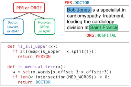
The key technical difficulty of weak supervision is deter-mining how to combine the labels of multiple sources that have different, unknown accuracies, may be correlated, and may label at different levels of granularity. In our experi-ence with users in academia and industry, the complexity of real world weak supervision sources makes this integration phase the key time sink and stumbling block. For example, if we are training a model to classify entities in text, we may have one available source of high-quality but coarse-grained labels (e.g. “Person” vs. “Organization”) and one source that provides lower-quality but finer-grained labels (e.g. “Doc-tor” vs. “Lawyer”); moreover, these sources might be corre-lated due to some shared component or data source (Bach et al. 2017; Varma et al. 2017). Handling such diversity re-quires addressing a core technical challenge: estimating the unknown accuracies of multi-granular and potentially corre-lated supervision sources without any labeled data.

To overcome this challenge, we proposeMeTaL, a frame-work for modeling and integrating weak supervision sources with different unknown accuracies, correlations, and gran-ularities. In MeTaL, we view each source as labeling one of several related sub-tasks of a problem—we refer to this as the multi-task weak supervision setting. We then show that given the dependency structure of the sources, we can use their observed agreement and disagreement rates to re-cover their unknown accuracies. Moreover, we exploit the relationship structure between tasks to observe additional cross-task agreements and disagreements, effectively pro-viding extra signal from which to learn. In contrast to pre-vious approaches based on sampling from the posterior of a graphical model directly (Ratner et al. 2016; Bach et al. 2017), we develop a simple and scalable matrix completion-style algorithm, which we are able to analyze by applying strong matrix concentration bounds (Tropp 2015). We use this algorithm to learn and model the accuracies of diverse weak supervision sources, and then combine their labels to produce training data that can be used to supervise arbitrary models, including increasingly popular multi-task learning models (Caruana 1993; Ruder 2017).

(2)

single-task setting (Ratner et al. 2016; 2018), and gener-ally considered conditiongener-ally-independent sources (Anand-kumar et al. 2014; Dawid and Skene 1979), we demonstrate that our multi-task aware approach leads to average gains of 4.1 points in accuracy in our experiments, and has at least three additional benefits. First, many dependency struc-tures between weak supervision sources may lead to non-identifiable models of their accuracies, where a unique solu-tion cannot be recovered. We provide a compiler-like check to establish identifiability—i.e. the existence of a unique set of source accuracies—for arbitrary dependency struc-tures, without resorting to the standard assumption of non-adversarial sources (Dawid and Skene 1979), alerting users to this potential stumbling block that we have observed in practice. Next, we provide sample complexity bounds that characterize the benefit of adding additional unlabeled data and the scaling with respect to the user-specified task and dependency structure. While previous approaches required thousands of sources to give non-vacuous bounds, we cap-ture regimes with small numbers of sources, better reflecting the real-world uses of weak supervision we have observed. Finally, we are able to solve our proposed problem directly with SGD, leading to over100_×faster runtimes compared to prior Gibbs-sampling based approaches (Ratner et al. 2016; Platanios et al. 2017), and enabling simple implementation using libraries like PyTorch.

We validate our framework on three fine-grained classi-fication tasks in named entity recognition, relation extrac-tion, and medical document classificaextrac-tion, for which we have diverse weak supervision sources at multiple levels of granularity. We show that by modeling them as label-ing hierarchically-related sub-tasks and utilizlabel-ing unlabeled data, we can get an average improvement of20.2points in accuracy over a traditional supervised approach,6.8points over a basic majority voting weak supervision baseline, and

4.1points over data programming (Ratner et al. 2016), an existing weak supervision approach in the literature that is not multi-task-aware. We also extend our framework to han-dle unipolar sources that only label one class, a critical as-pect of weak supervision in practice that leads to an average

2.8point contribution to our gains over majority vote. From a practical standpoint, we argue that our framework repre-sents an efficient way for practitioners to supervise mod-ern machine learning models, including new multi-task vari-ants, for complex tasks by opportunistically using the di-verse weak supervision sources available to them. To further validate this, we have released an open-source implementa-tion of our framework.1

2 Related Work

Our work builds on and extends various settings studied in machine learning.

Weak Supervision:We draw motivation from recent work which models and integrates weak supervision using gen-erative models (Ratner et al. 2016; 2018; Bach et al. 2017) and other methods (Guan et al. 2017; Khetan, Lipton, and

1

github.com/HazyResearch/metal

Anandkumar 2017). These approaches, however, do not han-dle multi-granularity or multi-task weak supervision, require expensive sampling-based techniques that may lead to non-identifiable solutions, and leave room for sharper theoreti-cal characterization of weak supervision stheoreti-caling properties. More generally, our work is motivated by a wide range of specific weak supervision techniques, which include tradi-tional distant supervision approaches (Mintz et al. 2009; Craven and Kumlien 1999; Zhang et al. 2017a; Hoffmann et al. 2011; Takamatsu, Sato, and Nakagawa 2012), co-training methods (Blum and Mitchell 1998), pattern-based supervi-sion (Gupta and Manning 2014; Zhang et al. 2017a), and feature-annotation techniques (Mann and McCallum 2010; Zaidan and Eisner 2008; Liang, Jordan, and Klein 2009).

Crowdsourcing: Our approach also has connections to the crowdsourcing literature (Karger, Oh, and Shah 2011; Dawid and Skene 1979), and in particular to spectral and method of moments-based approaches (Zhang et al. 2014; Dalvi et al. 2013a; Ghosh, Kale, and McAfee 2011; Anand-kumar et al. 2014). In contrast, the goal of our work is to support and explore settings not covered by crowdsourcing work, such as sources with correlated outputs, the proposed multi-task supervision setting, and regimes wherein a small number of labelers (weak supervision sources) each label a large number of items (data points). Moreover, we theoreti-cally characterize the generalization performance of an end model trained with the weakly labeled data.

Multi-Task Learning: Our proposed approach is mo-tivated by recent progress on multi-task learning mod-els (Caruana 1993; Ruder 2017; Søgaard and Goldberg 2016), in particular their need for multiple large hand-labeled training datasets. We note that the focus of our pa-per is on generating supa-pervision for these models, not on the particular multi-task learning model being trained, which we seek to control for by fixing a simple architecture in our ex-periments.

Our work is also related to recent techniques for estimat-ing classifier accuracies without labeled data in the pres-ence of structural constraints (Platanios et al. 2017). We use matrix structure estimation (Loh and Wainwright 2012) and concentration bounds (Tropp 2015) for our core results.

3 Programming Machine Learning with

Weak Supervision

(3)

Figure 1: A schematic of theMeTaLpipeline. To generate training data for anend model, such as a multi-task model as in our experiments, the user inputs atask graphGtaskdefining the relationships betweentask labelsY1, ..., Yt; a set ofunlabeled

data pointsX; a set ofmulti-task weak supervision sourcessi which each output a vector λi of task labels forX; and the

dependency structure between these sources,Gsource. We train alabel modelto learn the accuracies of the sources, outputting a vector of probabilistic training labelsY˜ for training the end model.

Figure 2: An example fine-grained entity classification prob-lem, where weak supervision sources label three sub-tasks of different granularities: (i)Personvs.Organization, (ii) Doctor vs. Lawyer (or N/A), (iii) Hospital vs. Office(orN/A). The example weak supervision sources use a pattern heuristic and dictionary lookup respectively.

rules to other models, and in this way can also be viewed as a pragmatic and flexible form of multi-sourcetransfer learn-ing.

In our experiences with users from science and industry, we have found it critical to utilize all available sources of weak supervision for complex modeling problems, includ-ing ones which label at multiple levels ofgranularity. How-ever, this diverse, multi-granular weak supervision does not easily fit into existing paradigms. We propose a formulation where each weak supervision source labels some sub-task of a problem, which we refer to as themulti-task weak super-visionsetting. We consider an example:

Example 1 A developer wants to train a fine-grained Named Entity Recognition (NER) model to classify men-tions of entities in the news (Figure 2). She has a multi-tude of available weak supervision sources which she be-lieves have relevant signal for her problem—for example, pattern matchers, dictionaries, and pre-trained generic NER taggers. However, it is unclear how to properly use and

com-bine them: some of them label phrases coarsely asPERSON versusORGANIZATION, while others classify specific fine-grained types of people or organizations, with a range of unknown accuracies. In our framework, she can repre-sent them as labeling tasks of different granularities—e.g. Y1 = _{Person,Org_},Y2 = _{Doctor,Lawyer,N/A_}, Y3 = {Hospital,Office,N/A}, where the label N/A applies, for example, when the type-of-person task is applied to an organization.

In our proposed multi-task supervision setting, the user specifies a set of structurally-relatedtasks, and then provides a set of weak supervision sources which are user-defined functions that either label each data point or abstain for each task, and may have some user-specified dependency struc-ture. These sources can be arbitrary black-box functions, and can thus subsume a range of weak supervision approaches relevant to both text and other data modalities, including use of pattern-based heuristics, distant supervision (Mintz et al. 2009), crowd labels, other weak or biased classifiers, declar-ative rules over unsupervised feature extractors (Varma et al. 2017), and more. Our goal is to estimate the unknown accu-racies of these sources, combine their outputs, and use the resulting labels to train an end model.

4 Modeling Multi-Task Weak Supervision

(4)

A Multi-Task Weak Supervision Estimator

Problem Setup Let X _{∈ X} be a data point and Y = [Y1, Y2, . . . , Yt]T be a vector of categoricaltask labels,Yi∈

{1, . . . , ki}, corresponding tottasks, where(X,Y)is drawn

i.i.d. from a distribution_D.2

The user provides a specification of how these tasks re-late to each other; we denote this schema as thetask struc-ture Gtask. The task structure expresses logical relation-ships between tasks, defining a feasible set of label vec-tors _Y, such that Y _{∈ Y}. For example, Figure 2 illus-trates a hierarchical task structure over three tasks of dif-ferent granularities pertaining to a fine-grained entity clas-sification problem. Here, the tasks are related by logical subsumption relationships: for example, ifY2 =DOCTOR, this implies that Y1 = PERSON, and that Y3 = N/A, since the task label Y3 concerns types of organizations, which is inapplicable to persons. Thus, in this task struc-ture,Y = [PERSON,DOCTOR,N/A]T _{is in}

Y while Y = [PERSON,N/A,HOSPITAL]T _{is not. While task structures}

are often simple to define, as in the previous example, or are explicitly defined by existing resources—such as ontologies or graphs—we note that if no task structure is provided, our approach becomes equivalent to modeling thettasks sepa-rately, a baseline we consider in the experiments.

In our setting, rather than observing the true label Y, we have access to mmulti-task weak supervision sources

si ∈ S which emit label vectorsλi that contain labels for

some subset of thettasks. Let0denote a null or abstaining label, and let thecoverage setτi ⊆ {1, . . . , t}be the fixed

set of tasks for which theith source emits non-zero labels, such thatλi∈ Yτi. For convenience, we letτ0={1, . . . , t} so that_Yτ0 =Y. For example, a source from our previous

example might have a coverage set τi = {1,3}, emitting

coarse-grained labels such as λi = [PERSON,0,N/A]T.

Note that sources often label multiple tasks implicitly due to the constraints of the task structure; for example, a source that labels types of people (Y2) also implicitly labels people vs. organizations (Y1 = PERSON), and types of organiza-tions (asY3=N/A). Thus sources tailored to different tasks still have agreements and disagreements; we use this addi-tionalcross-tasksignal in our approach.

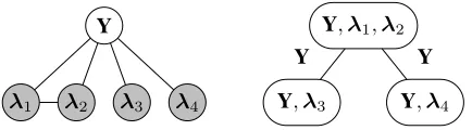
The user also provides the conditional dependency struc-ture of the sources as a graphGsource = (V, E), whereV = {Y,λ1,λ2, . . . ,λm}(Figure 3). Specifically, if(λi,λj)is

not an edge inGsource, this means thatλiis independent of

λj conditioned onYand the other source labels. Note that

if Gsource is unknown, it can be estimated using statistical techniques such as (Bach et al. 2017). Importantly, we do not know anything about the strengths of the correlations in

Gsource, or the sources’ accuracies.

Our overall goal is to apply the set of weak supervi-sion sourcesS ={s1, . . . , sm}to an unlabeled datasetXU

consisting ofndata points, then use the resulting weakly-labeled training set to supervise anend modelfw:X 7→ Y

(Figure 1). This weakly-labeled training set will contain

2

The variables we introduce throughout this section are sum-marized in a glossary in the Appendix, which can be accessed at https://arxiv.org/abs/1810.02840.

Y

λ1 λ2 λ3 λ4

Y,λ1,λ2

Y,λ3 Y,λ4

Y Y

Figure 3: An example of a weak supervision source de-pendency graph Gsource (left) and its junction tree repre-sentation (right), where Yis a vector-valued random vari-able with a feasible set of values, Y _{∈ Y}. Here, the out-put of sources 1 and 2 are modeled as dependent condi-tioned onY. This results in a junction tree with singleton separator sets, Y. Here, the observable cliques are O =

{λ1,λ2,λ3,λ4,_{λ1,λ2}} ⊂ C.

overlapping and conflicting labels, from sources with un-known accuracies and correlations. To handle this, we will learn alabel modelPµ(Y|λ), parameterized by a vector of

source correlations and accuracies µ, which for each data pointX takes as input the noisy labelsλ =_{λ1, . . . ,λm}

and outputs a single probabilistic label vectorY. Succinctly,˜ given a user-provided tuple(XU, S, Gsource, Gtask), our key technical challenge is recovering the parametersµwithout access to ground truth labelsY.

Modeling Multi-Task Sources To learn a label model over multi-task sources, we introduce sufficient statistics over the random variables in Gsource. Let _C be the set of cliques in Gsource, and define an indicator random variable for the event of a cliqueC∈ Ctaking on a set of valuesyC:

ψ(C, yC) =1{∩i∈CVi= (yC)i},

where(yC)i∈ Yτi. We defineψ(C)∈ {0,1}

Q

i∈C(|Yτi|−1) as the vector of indicator random variables for all combina-tions of all but one of the labels emitted by each variable in cliqueC—thereby defining a minimal set of statistics—and defineψ(C)accordingly for any set of cliquesC_{⊆ C}. Then

µ=E[ψ(C)]is the vector of sufficient statistics for the label model we want to learn.

We work with two simplifying conditions in this section. First, we consider the setting whereGsource istriangulated and has a junction tree representation with singleton separa-tor sets. If this is not the case, edges can always be added toGsource to make this setting hold; otherwise, we describe how our approach can directly handle non-singleton separa-tor sets in the Appendix.

Second, we use a simplifiedclass-conditional model of the noisy labeling process, where we learn one accuracy pa-rameter for each label value λi that each sourcesi emits.

This is equivalent to assuming that a source may have a dif-ferent accuracy on each difdif-ferent class, but that if it emits a certain label incorrectly, it does so uniformly over the differ-ent true labelsY. This is a more expressive model than the commonly considered one, where each source is modeled by a single accuracy parameter, e.g. in (Dawid and Skene 1979; Ratner et al. 2016), and in particular allows us to capture the

(5)

Our Approach The chief technical difficulty in our prob-lem is that we do not observeY. We overcome this by ana-lyzing the covariance matrix of an observable subset of the cliques inGsource, leading to a matrix completion-style ap-proach for recovering µ. We leverage two pieces of infor-mation: (i) the observability ofpart of Cov[ψ(_C)], and (ii) a result from (Loh and Wainwright 2012) which states that the inverse covariance matrixCov[ψ(_C)]−1is structured ac-cording toGsource, i.e., if there is no edge betweenλiandλj

inGsource, then the corresponding entries are 0.

We start by considering two disjoint subsets of_C: the set of observable cliques,O _{⊆ C}—i.e., those cliques not con-tainingY—and the separator set cliques of the junction tree, S ⊆ C. In the setting we consider here,_S =_{Y_}(see Fig-ure 3). We then write the covariance matrix of the indicator variables forO∪ S,Cov[ψ(O∪ S)], in block form, similar to (Chandrasekaran, Parrilo, and Willsky 2010), as:

Cov[ψ(O_{∪ S})]_≡Σ =

ΣO ΣOS ΣT

OS ΣS

(1)

and similarly define its inverse:

K= Σ−1₌

KO KOS KT

OS KS

(2)

Here, ΣO = Cov[ψ(O)] ∈ RdO×dO is the observable block of Σ, wheredO = PC∈O

Q

i∈C(|Yτi| − 1). Next, ΣOS = Cov[ψ(O), ψ(S)] is the unobserved block which

is a function ofµ, the label model parameters that we wish to recover. Finally,ΣS = Cov[ψ(S)] = Cov[ψ(Y)] is a function of the class balanceP(Y).

We make two observations aboutΣS. First, while the full form ofΣS is the covariance of the_{|Y| −}1indicator vari-ables for each individual value ofYbut one, given our sim-plified class-conditional label model, we in fact only need a single indicator variable forY(see Appendix); thus,ΣS is a scalar. Second,ΣS is a function of the class balanceP(Y), which we assume is either known, or has been estimated ac-cording to the unsupervised approach we detail in the Ap-pendix. Thus, givenΣO andΣS, our goal is to recover the

vectorΣOS from which we can recoverµ.

Applying the block matrix inversion lemma, we have:

KO = Σ−1O +cΣ −1

O ΣOSΣTOSΣ−1O , (3)

where c = ΣS₋ΣT OSΣ

−1 O ΣOS

−1

∈ R+. Let z = √_cΣ−1

O ΣOS; we can then express (3) as: KO = Σ−1O +zz

T ₍₄₎

The right hand side of (4) consists of an empirically ob-servable term, Σ−1_O , and a rank-one term, zzT_{, which we}

can solve for to directly recoverµ. For the left hand side, we apply an extension of Corollary 1 from (Loh and Wain-wright 2012) (see Appendix) to conclude thatKOhas

graph-structured sparsity, i.e., it has zeros determined by the struc-ture of dependencies between the sources in Gsource. This suggests an algorithmic approach of estimatingz as a ma-trix completion problem in order to recover an estimate of

µ(Algorithm 1). In more detail: letΩbe the set of indices

(i, j)where(KO)i,j = 0, determined byGsource, yielding a

system of equations,

0 = (Σ−1_O )i,j+ zzT

i,j for(i, j)∈Ω, (5)

which is now a matrix completion problem. Define_||A_||_Ωas the Frobenius norm ofAwith entries not inΩset to zero; then we can rewrite (5) as

Σ−1_O +zzT

_Ω = 0. We solve

this equation to estimatez, and thereby recoverΣOS, from

which we can directly recover the label model parametersµ

algebraically.

Checking for Identifiability A first question is: which dependency structures Gsource lead to unique solutions for

µ? This question presents a stumbling block for users, who might attempt to use non-identifiable sets of correlated weak supervision sources.

We provide a simple, testable condition for identifiability. LetGinv be the inverse graph ofGsource; note thatΩis the edge set of Ginv expanded to include all indicator random variablesψ(_C). Then, letMΩbe a matrix with dimensions |Ω_{| ×}dO such that each row inMΩcorresponds to a pair (i, j)∈Ωwith1’s in positionsiandjand 0’s elsewhere.

Taking the log of the squared entries of (5), we get a sys-tem of linear equationsMΩl =qΩ, whereli = log(zi2)and q(i,j)= log(((Σ−1O )i,j)2). Assuming we can solve this

sys-tem (which we can always ensure by adding sources; see Appendix), we can uniquely recover the z2

i, meaning our

model is identifiableup to sign. Given estimates of the z2

i, we can see from (5) that the

sign of a singlezidetermines the sign of all otherzj

reach-able fromzi inGinv. Thus to ensure a unique solution, we

only need to pick a sign for each connected component in Ginv. In the case where the sources are assumed to be independent, e.g., (Dalvi et al. 2013b; Zhang et al. 2014; Dawid and Skene 1979), it suffices to make the assumption that the sources areon averagenon-adversarial; i.e., select the sign of thezithat leads to higher average accuracies of

the sources. Even a single source that is conditionally in-dependent from all the other sources will cause Ginv to be fully connected, meaning we can use this symmetry break-ing assumption in the majority of cases even with corre-lated sources. Otherwise, a sufficient condition is the stan-dard one of assuming non-adversarial sources, i.e. that all sources have greater than random accuracy.

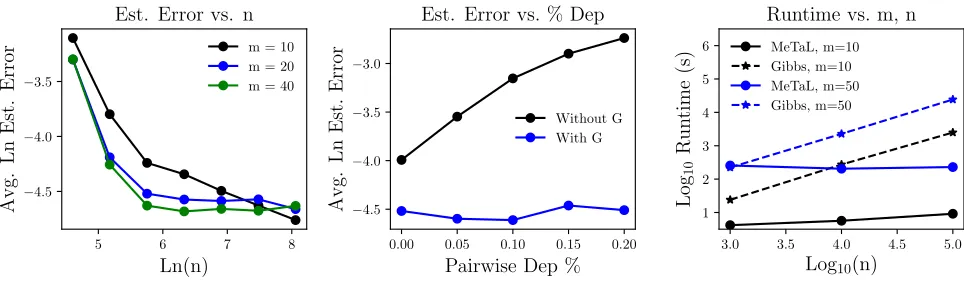
Source Accuracy Estimation Algorithm Now that we know when a set of sources with correlation structureGsource is identifiable, yielding a unique z, we can estimate the accuracies µ using Algorithm 1. We also use the func-tion ExpandTied, which is a simple algebraic expansion of tied parameters according to the simplified class-conditional model used in this section; see Appendix for details. In Fig-ure 4, we plot the performance of our algorithm on syn-thetic data, showing its scaling with the number of unla-beled data pointsn, the density of pairwise dependencies in

(6)

5 6 7 8 Ln(n) −4.5 −4.0 −3.5 Avg. Ln Est. Error

Est. Error vs. n

m = 10 m = 20 m = 40

0.00 0.05 0.10 0.15 0.20

Pairwise Dep % −4.5 −4.0 −3.5 −3.0 Avg. Ln Est. Error

Est. Error vs. % Dep

Without G With G

3.0 3.5 4.0 4.5 5.0

Log10(n) 1 2 3 4 5 6 Log 10 Run time (s)

Runtime vs. m, n

MeTaL, m=10 Gibbs, m=10 MeTaL, m=50 Gibbs, m=50

Figure 4: (Left) Estimation error_||µˆ₋µ∗

||decreases with increasingn. (Middle) GivenGsource, our model successfully recovers the source accuracies even with many pairwise dependencies among sources, where a naive conditionally-independent model fails. (Right) The runtime ofMeTaLis independent ofnafter an initial matrix multiply, and can thus be multiple orders of magnitude faster than Gibbs sampling-based approaches (Ratner et al. 2016).

Algorithm 1 Source Accuracy Estimation for Multi-Task Weak Supervision

Input:Observed labeling ratesEˆ[ψ(O)]and covariance

ˆ

ΣO; class balanceEˆ[ψ(Y)]and varianceΣS; correlation sparsity structureΩ

ˆ

z_←argmin_z

Σˆ −1 O +zz

T _Ω ˆ

c_←Σ−1_S (1 + ˆzT_Σˆ

Oz)ˆ,ΣˆOS ←ΣˆOz/ˆ

√

ˆ c ˆ

µ0

←ΣÔS+ Ê[ψ(Y)] Ê[ψ(O)] returnExpandTied(ˆµ0₎

Theoretical Analysis: Scaling with Diverse

Multi-Task Supervision

Our ultimate goal is to train anend modelusing the source labels, denoised and combined by the label model µˆ we have estimated. We connect the generalization error of this end model to the estimation error of Algorithm 1, ultimately showing that the generalization error scales asn−1

2, where

nis the number of unlabeled data points. This key result es-tablishes the same asymptotic scaling as traditionally super-vised learning methods, but with respect tounlabeleddata points.

Let Pˆµ( ˜Y | λ) be the probabilistic label (i.e.

distribu-tion) predicted by our label model, given the source la-bels λ as input, which we compute using the estimated

ˆ

µ. We then train an end multi-task discriminative model

fw : X 7→ Y parameterized byw, by minimizing the

ex-pected loss with respect to the label model overnunlabeled data points. Let l(w, X,Y) = 1

t

Pt

s=1lt(w, X,Ys) be a

bounded multi-task loss function such that without loss of generalityl(w, X,Y)_≤1; then we minimize the empirical

noise aware loss:

ˆ

w=argmin_w 1

n n

X

i=1

EY˜∼Pˆµ(·|λ)

l(w, Xi,Y˜)

, (6)

and letw˜be thewthat minimizes the true noise-aware loss. This minimization can be performed by standard methods and is not the focus of our paper; let the solutionwˆ satisfy Ekwˆ−w˜k2≤γ. We make several assumptions, follow-ing (Ratner et al. 2016): (1) that for some label model param-etersµ∗_{, sampling}₍_λ_,_Y₎

∼Pµ∗(·)is the same as sampling

from the true distribution,(λ,Y)∼ D; and (2) that the task labelsYsare independent of the features of the end model

givenλsampled fromPµ∗(·), that is, the output of the

op-timal label model provides sufficient information to discern the true label. Then we have the following result:

Theorem 1 Letw˜ minimize the expected noise aware loss, using weak supervision source parametersµˆestimated with Algorithm 1. Letwˆminimize the empirical noise aware loss withEkwˆ−w˜k2 ≤ γ,w∗ = minwl(w, X,Y), and let the assumptions above hold. Then the generalization error is bounded by:

E[l( ˆw, X,Y)−l(w∗, X,Y)]≤γ+ 4|Y| ||µˆ−µ∗||.

Thus, to control the generalization error, we must control ||µˆ₋µ∗

||, which we do in Theorem 2:

Theorem 2 Letµˆ be an estimate ofµ∗ _{produced by} Algo-rithm 1 run overnunlabeled data points. Leta:= (dO

ΣS +

(dO

ΣS)

2_λ

max(KO))

1

2 andb:= kΣ

−1

O k

2

(Σ−1_O )min. Then, we have:

E[||µˆ−µ∗||]≤16(|Y| −1)d2O

r

32π

n abσmax(M + Ω)

×3pdOaλ−1min(ΣO) + 1

κ(ΣO) +λ−1min(ΣO)

.

Interpreting the Bound We briefly explain the key terms controlling the bound in Theorem 2; more detail is found in the Appendix. Our primary result is that the estimation error scales asn−1

2. Next,σmax(M+

Ω), the largest singular

value of the pseudoinverseM+

Ω, has a deep connection to

(7)

more information we have aboutGinv, and the easier it is to estimate the accuracies. Next,λmin(ΣO), the smallest

eigen-value of the observed covariance matrix, reflects the condi-tioning ofΣO; better conditioning yields easier estimation,

and is roughly determined by how far away from random guessing the worst weak supervision source is, as well as how conditionally independent the sources are.λmax(KO),

the largest eigenvalue of the upper-left block of the inverse covariance matrix, similarly reflects the overall conditioning ofΣ. Finally,(Σ−1O )min, the smallest entry of the inverse

ob-served matrix, reflects the smallest non-zero correlation be-tween source accuracies; distinguishing bebe-tween small cor-relations and independent sources requires more samples.

Extensions: Abstentions & Unipolar Sources

We briefly highlight two extensions handled by our approach which we have found empirically critical: handling absten-tions, and modelingunipolarsources.

Handling Abstentions. One fundamental aspect of the weak supervision setting is that sources may abstain from labeling a data point entirely—that is, they may have incom-plete and differing coverage (Ratner et al. 2018; Dalvi et al. 2013b). We can easily deal with this case by extending the coverage ranges_Yτi of the sources to include the vector of all zeros,~0, and we do so in the experiments.

Handling Unipolar Sources. Finally, we highlight the fact that our approach modelsclass conditional source accura-cies, in particular motivated by the case we have frequently observed in practice ofunipolar weak supervision sources, i.e., sources that each only label a single class or abstain. In practice, we find that users most commonly use such unipo-lar sources; for example, a common template for a heuristic-based weak supervision source over text is one that looks for a specific pattern, and if the pattern is present emits a spe-cific label, else abstains. As compared to prior approaches that did not model class-conditional accuracies, e.g. (Ratner et al. 2016), we show in our experiments that we can use our class-conditional modeling approach to yield an improve-ment of2.8points in accuracy.

5 Experiments

We validate our approach on three fine-grained classification problems—entity classification, relation classification, and document classification—where weak supervision sources are available at both coarser and finer-grained levels (e.g. as in Figure 2). We evaluate the predictive accuracy of end models supervised with training data produced by several approaches, finding that our approach outperforms tradi-tional hand-labeled supervision by 20.2 points, a baseline majority vote weak supervision approach by6.8points, and a prior weak supervision denoising approach (Ratner et al. 2016) that is not multi-task-aware by4.1points.

Datasets Each dataset consists of a large (3k-63k) amount of unlabeled training data and a small (200-350) amount of labeled data which we refer to as thedevelopment set, which we use for (a) a traditional supervision baseline, and (b) for hyperparameter tuning of the end model (see Appendix).

The average number of weak supervision sources per task was13, with sources expressed as Python functions, averag-ing4lines of code and comprising a mix of pattern matching heuristics, external knowledge base or dictionary lookups, and pre-trained models. In all three cases, we choose the de-composition into sub-tasks so as to align with weak supervi-sion sources that are either available or natural to express.

Named Entity Recognition (NER): We represent a fine-grained named entity recognition problem— tagging entity mentions in text documents—as a hi-erarchy of three sub-tasks over the OntoNotes dataset (Weischedel et al. 2011): Y1 ∈ {Person,Organization_},

Y2 _∈ _{Businessperson,Other Person,N/A_}, Y3 _∈

{Company,Other Org,N/A_}, where again we use N/A

to represent “not applicable”.

Relation Extraction (RE):We represent a relation extrac-tion problem—classifying entity-entity relaextrac-tion menextrac-tions in text documents—as a hierarchy of six sub-tasks which ei-ther concern labeling the subject, object, or subject-object pair of a possible or candidate relation in the TACRED dataset (Zhang et al. 2017b). For example, we might label a relation as having a Person subject, Location object, and Place-of-Residence relation type.

Medical Document Classification (Doc): We represent a radiology report triaging (i.e. document classification) problem from the OpenI dataset (National Institutes of Health 2017) as a hierarchy of three sub-tasks: Y1 _∈

{Acute,Non-Acute_},Y2 ∈ {Urgent,Emergent,N/A_},Y3 ∈ {Normal,Non-Urgent,N/A_}.

End Model Protocol Our goal was to test the performance of a basic multi-task end model using training labels pro-duced by various different approaches. We use an architec-ture consisting of a shared bidirectional LSTM input layer with pre-trained embeddings, shared linear intermediate lay-ers, and a separate final linear layer (“task head”) for each task. Hyperparameters were selected with an initial search for each application (see Appendix), then fixed.

Core Validation We compare the accuracy of the end multi-task model trained with labels from our approach ver-sus those from three baseline approaches (Table 1):

• Traditional Supervision [Gold (Dev)]: We train the end model using the small hand-labeled development set. • Hierarchical Majority Vote[MV]: We use a hierarchical

majority vote of the weak supervision source labels: i.e. for each data point, for each task we take the majority vote and proceed down the task tree accordingly. This proce-dure can be thought of as a hard decision tree, or a cascade of if-then statements as in a rule-based approach. • Data Programming[DP]: We model each task separately

using the data programming approach for denoising weak supervision (Ratner et al. 2018).

(8)

NER RE Doc Average

Gold (Dev) 63.7_±2.1 28.4_±2.3 62.7_±4.5 51.6

MV 76.9_±2.6 43.9_±2.6 74.2_±1.2 65.0

DP (Ratner et al. 2016) 78.4_±1.2 49.0_±2.7 75.8_±0.9 67.7

MeTaL 82.2_±0.8 56.7_±2.1 76.6_±0.4 71.8

Table 1:Performance Comparison of Different Supervision Approaches.We compare the micro accuracy (avg. over 10 trials) with 95% confidence intervals of an end multi-task model trained using the training labels from the hand-labeled devel-opment set (Gold Dev), hierarchical majority vote (MV), data programming (DP), and our approach (MeTaL).

0 5 25 63

Unlabeled Datapointsn(Thousands) 63.7

77.2 80.6 82.2

Micro-Avg.

Accuracy

Accuracy vs.n(Log-Scale)

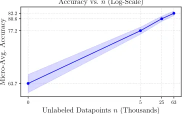
Figure 5: In the OntoNotes dataset, end model accuracy scales with the amount of availableunlabeleddata.

classification (for subtask-specific scores, see Appendix). We observe in Table 1 that our approach of leveraging multi-granularity weak supervision leads to large gains—

20.2 points over traditional supervision with the develop-ment set,6.8points over hierarchical majority vote, and4.1

points over data programming.

Ablations We examine individual factors:

Unipolar Correction:Modeling unipolar sources (Sec 4), which we find to be especially common when fine-grained tasks are involved, leads to an average gain of2.8points of accuracy inMeTaLperformance.

Joint Task Modeling:Next, we use our algorithm to es-timate the accuracies of sources for each task separately, to observe the empirical impact of modeling the multi-task set-ting jointly as proposed. We see average gains of 1.3 points in accuracy (see Appendix).

End Model Generalization:Though not possible in many settings, in our experiments we can directly apply the label model to make predictions. In Table 6, we show that the end model improves performance by an average 3.4 points in accuracy, validating that the models trained do indeed learn to generalize beyond the provided weak supervision. More-over, the largest generalization gain of 7 points in accuracy came from the dataset with the most available unlabeled data (n=63k), demonstrating scaling consistent with the predic-tions of our theory (Fig. 5). This ability to leverage addi-tional unlabeled data and more sophisticated end models are key advantages of the weak supervision approach in prac-tice.

# Train LM EM Gain

NER 62,547 75.2 82.2 7.0

RE 9,090 55.3 57.4 2.1

Doc 2,630 75.6 76.6 1.0

Figure 6: Using the label model (LM) predictions directly versus using an end model trained on them (EM).

6 Conclusion

We presented MeTaL, a framework for training models with weak supervision from diverse,multi-tasksources hav-ing different granularities, accuracies, and correlations. We tackle the core challenge of recovering the unknown source accuracies via a scalable matrix completion-style algorithm, introduce theoretical bounds characterizing the key scaling with respect to unlabeled data, and demonstrate empirical gains on real-world datasets. In future work, we hope to learn the task relationship structure and cover a broader range of settings where labeled training data is a bottleneck.

(9)

References

Anandkumar, A.; Ge, R.; Hsu, D.; Kakade, S. M.; and Tel-garsky, M. 2014. Tensor decompositions for learning latent variable models. The Journal of Machine Learning Research

15(1):2773–2832.

Bach, S. H.; He, B.; Ratner, A. J.; and R´e, C. 2017. Learning the structure of generative models without labeled data.

Blum, A., and Mitchell, T. 1998. Combining labeled and unlabeled data with co-training.

Caruana, R. 1993. Multitask learning: A knowledge-based source of inductive bias.

Chandrasekaran, V.; Parrilo, P. A.; and Willsky, A. S. 2010. Latent variable graphical model selection via convex opti-mization. InCommunication, Control, and Computing (Allerton), 2010 48th Annual Allerton Conference on, 1610–1613. IEEE. Craven, M., and Kumlien, J. 1999. Constructing biolog-ical knowledge bases by extracting information from text sources.

Dalvi, N.; Dasgupta, A.; Kumar, R.; and Rastogi, V. 2013a. Aggregating crowdsourced binary ratings.

Dalvi, N.; Dasgupta, A.; Kumar, R.; and Rastogi, V. 2013b. Aggregating crowdsourced binary ratings.

Dawid, A. P., and Skene, A. M. 1979. Maximum likelihood estimation of observer error-rates using the em algorithm.

Applied statistics20–28.

Ghosh, A.; Kale, S.; and McAfee, P. 2011. Who mod-erates the moderators?: Crowdsourcing abuse detection in user-generated content.

Guan, M. Y.; Gulshan, V.; Dai, A. M.; and Hinton, G. E. 2017. Who said what: Modeling individual labelers im-proves classification.arXiv preprint arXiv:1703.08774.

Gupta, S., and Manning, C. D. 2014. Improved pattern learning for bootstrapped entity extraction.

Hoffmann, R.; Zhang, C.; Ling, X.; Zettlemoyer, L.; and Weld, D. S. 2011. Knowledge-based weak supervision for information extraction of overlapping relations.

Karger, D. R.; Oh, S.; and Shah, D. 2011. Iterative learning for reliable crowdsourcing systems.

Khetan, A.; Lipton, Z. C.; and Anandkumar, A. 2017. Learning from noisy singly-labeled data. arXiv preprint arXiv:1712.04577.

Liang, P.; Jordan, M. I.; and Klein, D. 2009. Learning from measurements in exponential families.

Loh, P.-L., and Wainwright, M. J. 2012. Structure estima-tion for discrete graphical models: Generalized covariance matrices and their inverses.

Mann, G. S., and McCallum, A. 2010. Generalized ex-pectation criteria for semi-supervised learning with weakly labeled data.JMLR11(Feb):955–984.

Mintz, M.; Bills, S.; Snow, R.; and Jurafsky, D. 2009. Dis-tant supervision for relation extraction without labeled data.

National Institutes of Health. 2017. Open-i.

Platanios, E.; Poon, H.; Mitchell, T. M.; and Horvitz, E. J. 2017. Estimating accuracy from unlabeled data: A proba-bilistic logic approach.

Ratner, A. J.; De Sa, C. M.; Wu, S.; Selsam, D.; and R´e, C. 2016. Data programming: Creating large training sets, quickly.

Ratner, A.; Bach, S.; Ehrenberg, H.; Fries, J.; Wu, S.; and R´e, C. 2018. Snorkel: Rapid training data creation with weak supervision.

Ruder, S. 2017. An overview of multi-task learning in deep neural networks. CoRRabs/1706.05098.

Søgaard, A., and Goldberg, Y. 2016. Deep multi-task learn-ing with low level tasks supervised at lower layers.

Takamatsu, S.; Sato, I.; and Nakagawa, H. 2012. Reducing wrong labels in distant supervision for relation extraction. Tropp, J. A. 2015. An introduction to matrix concentra-tion inequalities. Foundations and TrendsR in Machine Learn-ing8(1-2):1–230.

Varma, P.; He, B. D.; Bajaj, P.; Khandwala, N.; Banerjee, I.; Rubin, D.; and R´e, C. 2017. Inferring generative model structure with static analysis.

Weischedel, R.; Hovy, E.; Marcus, M.; Palmer, M.; Belvin, R.; Pradhan, S.; Ramshaw, L.; and Xue, N. 2011. Ontonotes: A large training corpus for enhanced processing.Handbook of Natural Language Processing and Machine Translation. Springer. Xiao, T.; Xia, T.; Yang, Y.; Huang, C.; and Wang, X. 2015. Learning from massive noisy labeled data for image classi-fication.

Zaidan, O. F., and Eisner, J. 2008. Modeling annotators: A generative approach to learning from annotator rationales. Zhang, Y.; Chen, X.; Zhou, D.; and Jordan, M. I. 2014. Spectral methods meet em: A provably optimal algorithm for crowdsourcing.