Volume 04 Issue 05 May- 2019, Page No.-597-612
DOI:10.31142/etj/v4i5.03, I.F. - 4.449
© 2019, ETJ
597
Abelardo Buentello-Duque
1, ETJ Volume 4 Issue 05 May 2019
Wind Farm Layout Optimization Using Genetic Algorithms and Design of
Experiments
Abelardo Buentello-Duque
1, Salvador Hernández-González
2, José A. Jiménez-García
3,
Vicente Figueroa-Fernández
4, Moisés Tapia-Esquivias
51,2,3,4&5Tecnológico Nacional de México en Celaya, Department of Industrial Engineering; Av. García Cubas 1200, Esquina
Ignacio Borunda, Celaya, Gto. México. Tel. 01 (461)61 17575
Abstract
: Wind power has become the renewable energy with more participation in countries looking for environmental sustainability. Wind power is transformed into electric power by means of wind turbines, which are generally grouped in wind farms to exploit the relative benefits to economies of scale. The efficient design of a wind farm requires a set of wind turbines to be distributed to produce the maximum amount of installed energy. One of the typical factors to be considered for the optimal design of a wind farm is the interaction between the fields of operation of the wind turbines or the wake effect; wake effect provokes a considerable loss of power, so it is important when designing a wind farm to consider said wake effects in such a way as to maximize the expected energy production. The wind farm layout optimization problem is considered an NP-hard optimization problem, as there is no algorithm that can solve it in polynomial computation time. This research proposes the implementation of an evolutionary metaheuristic to find the optimal allocation of turbines in wind farms, considering the wake effect. In order to find those parameters of the genetic algorithm that provide high quality solutions in reasonable computation time, a factorial experimental design 25 was used. The results of the solved instances demonstrated that the metaheuristic method and the design of experiments technique provide different configurations that improve up to 1% in both utility and power generation than the previous configurations proposed in the literature in reasonable computing times.Keywords:
wind farm, wake effect, artificial intelligence, combinatorial optimization, genetic algorithms, design of experiments, renewable energy, metaheuristic.I. INTRODUCTION
Wind power is considered to be the fastest growing source of renewable energy since worldwide production grew significantly between 2005 and 2008, reaching 121. 2 GW of total installed capacity. Which has made this green energy an extremely interesting topic in the last few years. Environmental sustainability demands a considerable reduction in the use of fossil fuels, which are extremely contaminating and unsustainable, so ambitious plans have been proposed for the production of green energy, including wind power [1]. Wind power is transformed into electric power by means of wind turbines, which are generally grouped in wind farms to exploit the relative benefits to economies of scale, such as lower costs of installation and maintenance [2]. A wind farm’s design is an important component in guaranteeing the profitability of a wind farm project. A bad design or an unsuitable wind turbine layout in wind farms might result in a lower production of wind power compared to expected production; higher maintenance costs; among other unsatisfactory aspects [3].
The wind farm layout optimization problem consists of finding an optimal allocation of wind turbines on a particular site that maximizes energy production. In practice
598
Abelardo Buentello-Duque
1, ETJ Volume 4 Issue 05 May 2019
One of the typical factors to be considered for theoptimal design of a wind farm is the interaction between the fields of operation of the wind turbines, known as the wake effect, which is treated as a non-linear phenomenon. According to estimates, the average loss of power resulting from the wake effect between turbines in large offshore wind farms is about 10-20% of the total energy production [9]. However, said rates of power loss also, to a greater extent, depend of the particular conditions and characteristics of the wind farm such as: wind speed, distance between wind turbines, the model of wind turbines, etc.
Wake effect is an interaction-derived phenomenon that refers the situation that arises when two neighboring wind turbines are located at a certain distance, and a certain wind current comes from a dominant direction with a certain initial speed and this current interacts with the first upstream wind turbine, said wind turbine creates turbulence in the wind arising from its absorption of kinetic energy, causing said wind to loss considerable speed and force. The weakened wind, as it continues its course will be absorbed by a second wind turbine downstream, which shall have at its disposal less kinetic energyto operate, causing a notable drop in the rated output (Megawatt, Kilowatt, etc.) of its power production.
Therefore, on a large wind farm wind, wake effect provokes a considerable loss of power [10], so it is extremely important when designing a wind farm to minimize said wake effects in such a way as to maximize the expected energy production.
The modeling of the wake effect phenomenon fulfills an important function in understanding the behavior of wind turbulence when it interacts with a set of wind turbines on a wind farm. It also makes it possible to quantify the wind speed deficits created by said effects in order to later calculate the loss of power corresponding to the incident speed deficits on each one of the affected wind turbines. In [4], a compilation and review of the different wake effect models in existence was done, comparing the different models to demonstrate that the Jensen model is a good option for solving the wind farm layout optimization problem, owing to its simplicity and relatively high level of precision. For the purpose of this paper, we only consider the Jensen model for calculating the speed deficits caused by wake effects among two or more wind turbines, therefore the total of these deficits throughout the wind farm is considered to be the sum of the speed deficits present. In the wind farm optimization problem, a distant wake effect is more significant than a nearby wake effect [4]. Despite the Jensen model being an approximation of the real environment, it gives satisfactory results for the purposes of this research.
One main advantage of this model is that it offers the possibility of implicitly dealing with a considerable number
of wind scenarios, something that, for practical effects, is a necessity [1].
Therefore, the purpose of this paper is to optimize the positions or locations of the turbines in such a way that we get an optimal layout or design of the wind farm, ensuring that the maximum amount of installed power is produced by the wind farm, taking the reductions of energy caused by the wake effect into account. We propose to achieve this by using a metaheuristic approach, specifically the implementation of genetic algorithms, which in turn is combined with the design of experiments technique to provide good quality solutions within a reasonable computation time for large-scale wind farm layout scenarios.
II. MATERIAL and METHODS (BODY TEXT)
The first part of this section gives a brief explanation of the construction phases of a wind farm project. The second part sets forth the discretization strategy to reduce the problem's complexity. A brief explanation of wind turbines is given in the third part. The fourth part presents the wake effect model we used. While lastly, the fifth part of this section shows the Genetic Algorithm adaptation used to solve this problem. Likewise, a factorial experimental design is at two levels is carried out with the algorithm to find the proper parameters that will provide high quality solutions for the instances considered in this research in a reasonable computation time. The experimental design and its results are presented in the results section. Design-Expert (Version 7.1.6 Trial) software is used for the experiment.
CONSTRUCTION of a WIND FARM
This section briefly explains the stages in the construction of a wind farm project. It is worth mentioning that, for the purposes of this paper, we have excluded the development of the first two stages as we are focusing on optimizing: installed wind farms, those that have at least an initial design or layout or those that are at the stage of planning their installation. In other words, this research is mainly focused on the third stage.
The first phase in the construction of a wind farm is to find a windy site to ensure the profitability of the project. According to [11], there are two types of wind farms: land-based and offshore ones. This research only considers wind farms built on land.
In the second stage the owner of the land is contacted to draw up the corresponding agreements. In parallel with this stage, the wind farm developers install measurement devices and determine the distribution of the wind. Furthermore, the number of turbines and the models to be installed are defined in this stage.
599
Abelardo Buentello-Duque
1, ETJ Volume 4 Issue 05 May 2019
WIND FARM DISCRETIZATION
In order to reduce the complexity of the wind farm design optimization problem and thus get good quality solutions, discretization is applied to the wind farm by means of small squares or small rectangles. This is because this paper only considers totally flat wind farms that are either square or rectangular and are divided into small square or rectangular cells. Likewise, this research only considers wind turbines that are all of the same height. The centroids or points inside the squares represent the possible locations where a turbine could be installed.
Figure 1 presents a proposed design (scenario) for a wind farm of 600 m x 600 m, showing its discretization for the purpose of finding the precise center of each square, the possible location or ring where a wind turbine could be assigned or installed. For this specific design, we have a predefined set of 25 possible discrete locations with dimensions of 120 m x 120 m, in 11 of which a wind turbine is allocated or installed (represented by red filled in rings). For this scenario in particular, the number of possible combinations or ways of designing the wind farm amounts to 4,457,400. A specific wind with an initial speed and a dominant North-to-South direction is involved in the proposed wind farm scenario. These discretization strategy is very useful as, if it is not discretized, the algorithm used would take a very long time to find a solution within a continuous solution space.
Figure 1. Discrete wind farm
WIND TURBINES
Wind turbines are electrical devices that extract kinetic energy from the wind to transform mechanical energy into electric power.
The main characteristics of a wind turbine that are linked to wind farm design optimization are given in Table 1.
Table 1. Main characteristics and nomenclature
Characteristic Nomenclature
Cut-in speed
Cut-out speed
Rotor diameter d
Hub height Z
Rated speed -
Rated power -
Power curve -
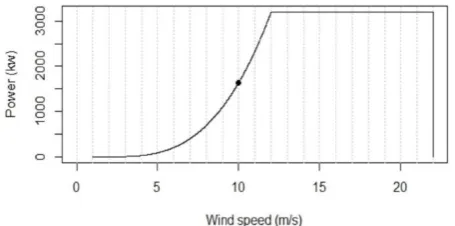
When a wind impacts on a turbine and its speed is higher than , the blades of the turbines start to turn and generate power (energy). The power produced ascends to the cube at the rate of the wind speed until the wind speed reaches the rated speed, at which point the wind turbine’s control system adjust the rhythm of the blades for the power that is produced to be uniform and equivalent to the rated power. When the wind speed reaches , the wind turbine automatically stops, owing to the fact if it works at a speed that is equal to or greater than this speed, its electrical and/or mechanical components will be damaged. Another of the significant main characteristics is the power curve, which provides the power produced at every wind speed between and . Figure 2 shows an example of the power curve of a SENVION wind turbine ( = 3 m/s, = 22 m/s, rated power = 3,200 kW, rated speed = 12 m/s).
Figure 2. Power curve of a SENVION Model 3.2M114 NES wind turbine
WAKE EFFECT
600
Abelardo Buentello-Duque
1, ETJ Volume 4 Issue 05 May 2019
available models, which are divided into two main groups:Kinematic Models and Wind Farm Models. According to [4], the model that stand out is the Jensen model, which belongs to the family of Kinematic Models. For this paper, we consider the Jensen model that is proposed in [2], which, in turn, is a model equivalent to the one proposed in [12].
The use of this model is justified as a variety of s studies have demonstrated that the model is computationally efficient and has a high degree of precision for the purposes it has been set.
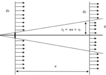
The model consists of a cone with a linear expansion of the diameter of the wake effect and a linear decrease of the wind speed deficit inside wake effect. For a better explanation of the model, see Figure 3.
Figure 3. Schematic representation of the wake effect
Figure 3 shows a wind incident from left to right at a certain speed and interact with a turbine (represented by a small vertical line in bold on the left of the Figure). The radius of this turbine’s rotor is . At a particular distance x
in the same direction as the wind, the wind speed is U and the radius of the wake (initially rr) is deduced as
.
Scalar α determines that the wake effect expands as fast as it advances in relation to the distance and this is denoted as:
(1)
where z is the hub height of the turbine producing the wake effect and z0 is a constant, known as surface roughness, that depends on the characteristics of the surface of the land. Let be I the position of the turbine that creates the wake effect, j the position affected by position i, the pure incident wind speed (without turbulence), and the wind speed available at j. Then:
(2)
where is the speed deficit that is induced at position
j by the wake effect created by i. therefore vdij is calculated suing the following equation:
(3)
The term a that appears in the numerator is known as the axial induction factor and is calculated as follows:
(4)
In (4) the term is the constant thrust coefficient, which assesses the proportion of energy captured when the wind passes through the blades of the wind turbine [13]. The manufacturers of wind turbines normally provide data and information about the thrust coefficient.
In (3), the term rd, that is presented in the denominator, is called downstream rotor radius (radius of the downstream wake effect) and is calculated with the following expression:
(5)
The term is the distance between positions iand j.
As most the wind farms have a large number of wind turbines installed, the wake effect can be interwoven and accumulated. These accumulations of wake effect may affect one or more downstream turbines at the same time. In the Jensen model, the total speed deficit in a position
j that is affected by more wake effects is obtained by using the following expression:
(6)
where ) is the set of wind turbines that affect position j
with a wake effect. Therefore, is substituted in (2) in
the place of to calculate .
GENETIC ALGORITHM
601
Abelardo Buentello-Duque
1, ETJ Volume 4 Issue 05 May 2019
chromosomes. Each chromosome is an individual thatrepresents a design or layout of the wind farm being studied. The set of individuals is called the population.
The genetic algorithm mainly works with three genetic operators: selection, crossover and mutation. The selection operator consists of selecting and retaining a certain number of individuals that can generate better fitness values in every iteration (generation) according to the predefined selection probability or the chosen selection method. In the optimization package used in this research, different adjustments can be made to the parameters or input variables such as, for example, in the “selstate” selection variable where the possible input values or selection methods are “FIX” and “VAR”. When the algorithm performs the selection process, based on the fitness values, it eliminates the four worst individuals from the population. Once the individuals (parents) have been selected, the algorithm will perform the crossover on the basis of probability or the chosen crossover method. The crossover operator does the job of combining the individuals’ genetic information in order to be able to procreate children from the selected parents and using it to find individuals that are fitter or better assessed in terms of fitness. Likewise, the crossover method’s input variable “crossPart1” can be defined as “EQU” or “RAN” as desired. Likewise, the mutation operator is performed after the crossover, whose function is to increase the diversity of the individuals to avoid a premature convergence on local optima. In the Rstudio package, the parameter for the mutation rate can also be adjusted in accordance with the percentage of individuals to be mutated in each iteration. After selection, crossover and mutation, the fitter individuals or the ones with better results are transferred to the next one to the next generation. At the same time, the individuals that are less fit are removed. The elitist selection may also be considered in the algorithm. If the elitism method is activated, the “nelit” input variable determines the number of individuals that must be saved to form part of the elite population. This elite population is not saved separately. However their fitness values increase by a factor of 10, mainly to simplify implementation. The probability of these individuals being selected is, therefore, much higher than that of the rest of the individuals, although the selection process will still be random.
In [14] the characteristics and considerations of the selection, crossover, mutation and elitism methods considered in the algorithm package are explained in detail. Likewise, [14] gives a detailed description of other adjustable parameters in the package, that have nothing to do with the genetic algorithm but form an essential part of optimal wind farm design, such as: Grid Method and Surface Roughness.
Finally, the algorithm has two stopping criterion: the algorithm stops when the number of generations exceeds the predefined number of iterations in the “iteration” input
variable or when a wind farm design is found with 100% efficiency.
Equation (7) shows the objective function to be optimized where the fitness values of each one of the solutions (individuals) generated by the algorithm are assessed.
s.t.
Where:
: Instant power or energy generated by turbine j, owing to
the interference of i (continuous in units of power). = Total power produced (continuous in units of power). = Number of turbines to be installed.
Genetic Algorithm implementation strategy for the scenario proposed in section of Materials and Methods:
1. Randomly generating an initial population of individuals P that shall be called parents. In the package used, the algorithm randomly generates for the initial population of 100 individuals or chromosomes. Each individual consists of a binary chain of 25 positions or genes. Consider that a value of 1 in one position represents a turbine installed in the corresponding centroid and 0 another case. To locate a turbine in the discrete wind farm, the possible locations or centroids are enumerated in rows. Figure 4 shows an example of 5 randomly generated individuals (a-d), where each one corresponds to a specific wind farm design or layout.
Figure4. Randomly generated individuals for the initial population
2. Calculate the fitness function F(x)as per equation (7) for each one of the parents of P.
602
Abelardo Buentello-Duque
1, ETJ Volume 4 Issue 05 May 2019
shall be ordered from the lowest to the highest, bymeans of the following division:
.
4. While (according to the shutdown criteria).
5. Select a population for the operator of variation crossover: “FIX” Method or “VAR” Method. The Roulette Wheel Selection Method is used to select, according to the chosen selection method, the fitter individuals (parents) to create pairs and procreate the children.
6. Crossing the individuals (parents): “EQU” Method or “RAN” Method. Therefore, as per the selected method, two parents are chosen to share their genetic information. For example, Figure 5 shows two individuals presented in step 1.
Figure 5. Parents selected to share their genetic information in position 10 of the chromosome
The parents (a) and (b) will procreate two new children (A-D, C-B) with new genetic information, in other words, new chromosomes with shared genes. Figure 6 shows the new individuals (children) created from the parents.
Figure 6. New procreated individuals
7. Mutating the children at a certain rate of probability. According to [14], the mutation rate would have treated as fairly small, so a range of 0.01% to 0.10% is recommended and even complementing a fixed mutation rate with a variable mutation rate is also recommended. In the chromosome or binary chain of the child selected for mutation, a position will be chosen by random probability and the gene will be modified in said position. If it contained a value 0, this is changed to 1 and vice versa, as the case may be. Figure 7 gives an example of mutation in position 14 of child #1 procreated at step 6.The crossover and the mutation function change the number of wind turbines in the wind farms. However, the algorithm is designed to operate with a constant number of turbines. This occurs as the fitness value of an individual is the expected energy production.
Figure 7. Child #1 mutated in position 14
8. Calculate the fitness function F(x) of the procreated children. The proportional values obtained from the assessment of the objective function of the new individuals (children) shall be ordered from the lowest to the highest, by means of the following division:
.
9. Insert children in P. The strongest or fittest children will be replaced by weak parents, P will be constantly updated until the individual with the best fitness value assessed in the objective function is procreated. Let us call this individual the best solution phenotype. The algorithm produces the phenotype found in all the iterations.
Table 2 shows the Genetic Algorithm’s pseudocode.
Table 2. Genetic algorithm’s pseudocode
Genetic Algorithm
1: t← 0; /* Iteration counter */
2: initialize (P) /* Initialize the population */ 3: whilethere is no stopping criterion (t, P)do
4: Parents ← selection (P); /* Select parents */ 5: Children←reproduction (Parents) /* Crossover */ 6: mutation(Children) /* Mutate the children */ 7: evaluate(Children) /* Evaluate the children */ 8: newGeneration = replacement (P, Children)
/*replaces the population with the current */ 9: t ← t + 1 /* One more iteration */ 10: end while
11: Return: best solution found.
III. RESULTS and DISCUSSION
Two instances proposed in [14] are solved in this section. Case 1 corresponds to one medium instance. Case 2 corresponds to an instance of 100 possible locations and 30 turbines to be installed. Three varieties of Case 2 (Case 2(a), Case 2(b) and Case 2(c)) solved. The characteristics for each variant in Case 2 are given at the start of each subsection.
603
Abelardo Buentello-Duque
1, ETJ Volume 4 Issue 05 May 2019
fractional factorials. It was also decided to use 3 replicas toestimate the mean and standard deviation of the data obtained in the response variables when the treatments were run. Additionally, to justify the use of 3 replicates and 8 central points in the experiment, it was found in Minitab that the design power for both response variables considering this number of replicates and this number of central points is greater than 99%, so it is assumed that the probability of correctly finding a significant effect is greater than 99%.
The experimental design was applied to Case 1 and then we take the parameters that give the maximum energy for this instance and propose their use in the variants of Case 2. Table 3 shows the factors and levels of factors considered in the experiment. Figure 8 shows a fragment of the experiment done in Design-Expert. It is worth mentioning that the experiments were carried out in parallel computing with 2 cores in a computer with the following specifications: Intel(R) Core(TM) i5-7200U CPU @ 2.50GHz, 2701 Mhz, 2 main processors, 4 logical processors and installed physical memory (RAM) of 8GB.
Table 3. Factors, types and levels of factors for the experiment
Factor Name
Type Low
level
High level
Crossover method
Categoric EQU RAN
Selection method
Categoric FIX VAR
Elitism Categoric TRUE FALSE Mutation rate Numeric 0.01 0.1
Number of iterations
Numeric 50 100
Figure 8. Fragment of experiment 25 with 3 replicas and 8 center points
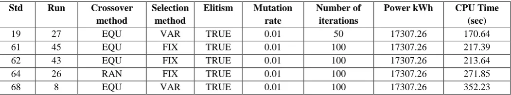
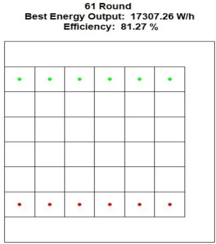
Therefore, having performed the experiment’s 104 total runs we discover that 5 runs or parameter configurations manage to reach the maximum expected energy for Case 1. The maximum expected energy for Case 1 is 17307.26 kWh. Table 4 shows the 5 runs in the experiment that achieve the maximum expected energy for the wind farm instance with its respective computation time. Note that standard runs 61 and 62 correspond to two replicas out of the three that were performed using that parameter configuration. The use of these 5 runs is proposed to optimize the variants of the instance in Case 2. To optimize the corresponding instances of Case 2 standard run 64 is especially used, changing the mutation rate to 0.006 so that the algorithm performs an efficient search.
Table 4. Configurations of the factors that achieved maximum expected energy in Case 1
Std Run Crossover
method
Selection method
Elitism Mutation rate
Number of iterations
Power kWh CPU Time
(sec)
19 27 EQU VAR TRUE 0.01 50 17307.26 170.64
61 45 EQU FIX TRUE 0.01 100 17307.26 217.39
62 43 EQU FIX TRUE 0.01 100 17307.26 213.64
64 26 RAN FIX TRUE 0.01 100 17307.26 271.85
68 8 EQU VAR TRUE 0.01 100 17307.26 352.23
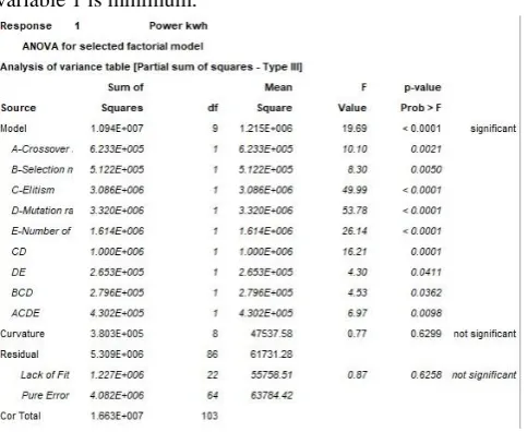
Likewise, as part of the factorial experiment developed in Design Expert, the Analisis of Variance (ANOVA) was performed for each one of the response variables considered: Energy and CPU Time. Figure 9 is the ANOVA Table corresponding to response number 1’s variable: Energy kWh. The ANOVA shows the factors and interactions that are significant or have an influence on this response variable. In this case, all the main factors (A, B, C, D and E) as well as the interactions CD, DE, BCD and ACDE are significant. Moreover, it is possible to appreciate that there is no evidence of curvature in the experimentation region.
604
Abelardo Buentello-Duque
1, ETJ Volume 4 Issue 05 May 2019
statistic is a measurement of the amount of variation or noisein the model, the desired value is 4 or higher. In this case, the Adeq Precision value is 11.504, which indicates that the amount of variation in the model corresponding to response variable 1 is minimum.
Figure 9. ANOVA for response variable 1: Energy
Table 5. Statistics corresponding to response variable 1: Energy
.6732
-adj .6390
Adeq Precision 11.504
Likewise, Analysis of Variance is performed for response variable number 2: CPU Time. Figure 10 gives the ANOVA table, which indicates that the main factors B and E together with their interaction have an influence on the CPU Time used by the algorithm. Likewise, the ANOVA reveals that there is no curvature in the experimentation region.
Table 6 provides the corresponding analysis statistics. In this case, the statistic indicates that the 85.77% of variability in CPU Time is explained by the factors that are included in the model. As the value and the -adj value do not dramatically differ, it is assumed that the appropriate factors have been included in the model. Lastly, the Adeq Precision statistic contains a value of 27.805, which indicates that the amount of variation in the model is minimum.
Figure 10. ANOVA for response variable 2: CPU Time
Table6. Statistics corresponding to response variable 2: CPU Time
.8577
-adj .8534
Adeq Precision 27.805
Case 1
Table 7 gives the input values corresponding to Case 1, which is proposed in [14]. To solve this case note that in Table 7 considered the parameters of standard run 61 that was presented in Table 4. Figure 11 shows the characteristics and dimensions of the wind farm to be optimized. Said figure shows a discrete wind farm with 36 squares, where every centroid of every square represents a possible location for a turbine. The dimension (resolution) of each square is 90m x 90m. In accordance with the input variable “n” that is specified in Table 7, 12 turbines that are planned to be installed in said wind farm. Figure 12 corresponds to the wind rose, according to the information included in “data.in” found in Table 7. The “data.in” information indicates the direction and speed with which the wind considered for this case is propagated. For this scenario, an incident wind is considered with a uniform direction of 0° (North-South) and a constant speed of 12 m/s.
Table 7. Input values for Case 1
Input Variable Value
n (Number of turbines to be
installed)
12
SurfaceRoughness(meters) 0.14
Rotor Radius(meters) 30
fcrR(value for grid spacing) 3
RotorHeight(meters) 60
referenceHeight(meters) 60
Iteration 100
Proportionality 1
mutr(Mutation rate) 0.01
vdirspe(wind speed and direction) data.in(12 m/s at
0°)
Topograp "FALSE"
Elitism "TRUE"
Nelit 6
Selstate “FIX”
crossPart1 “EQU”
605
Abelardo Buentello-Duque
1, ETJ Volume 4 Issue 05 May 2019
Figure11. Characteristics and dimensions of the wind farm to be optimized
Figure 12. Wind rose for Case 1
Therefore, considering all of the above, the best layout solution for this case is shown in Figure 13. This is considered to be the best possible solution as there is no other wind farm design or layout that provides a higher total amount of energy. Therefore, this solution is considered to be the best layout solution for Case 1. Likewise, it is possible to appreciate in Figure 13 the points inside the squares where the wind turbines are installed in accordance with the optimum solution found. The colors and values that are given under these points indicate the loss of power caused by the wake effect. The points where the energy deficits caused by the wake effect are weak are represented in green, while the points where the energy deficits caused by the wake effects are high are shown of red. Figure 13 also shows the minimum distance and the average distance at which all the turbines are to be found according to the solution that has been found. The CPU time that the algorithm invested in finding such solution, using parallel computing with 2 cores, was 227.67 seconds.
Figure 14 shows that, in iteration number 61, the algorithm converged on the best possible solution. Figure 15 shows the best evaluated individual or solution vector for Case 1, which agrees with the best wind turbine layout
presented in Figure 13. On that vector we can see a chromosome or individual with 36 positions. Each one of these positions represents a centroid or a possible location for a turbine so we have a solution vector with 12 1’s in total, which represents the total number of turbines planned to be installed.
Figure 16 shows the same solution found by the algorithm from a perspective is more real or similar to a wind farm. It is also possible to appreciate in said figure that the turbines shaded in green are the ones that are less affected by the wake effect, while those shaded in red are more affected by the wake effects.
Figure 17 reports the progress of the amount of energy produced in each one of the generations. In said figure, the maximum energy value achieved by an individual in each generation is represented by the color green, the average energy values by blue and the minimum energy values by red.
Figure 18 indicates the number of individuals from each population in all the generations. The numbers of individuals counted after the fitness, selection and crossover function. The number of individuals in each iteration is the same for both the fitness function and the crossover function. The black points represent the number of individuals after the fitness function, the red points the number of individuals after the selection function and the green points indicate the number of individuals once the crossover has been performed.
Figure 19 shows the evolution of the wind farm’s energy efficiencies during all the generations or iterations. The maximum values found for energy efficiency are represented by green, the average values by blue and the minimum values by red. Likewise, said figure shows the influence of mutation in terms of the energy efficiency values. The vertical black lines indicate the iterations where the variable mutation rate is used instead the fixed mutation rate. In this case, the algorithm resorted to the variable mutation rate 7 times to explore others corners of the feasible solution space.
Figure 20 shows the evolution of the wind farm’s energy efficiencies during all the generations. Vertical green lines are used to illustrate the generations where the percentage of selection was higher than 75%. According to Figure 18, some iterations had a fairly low number of individuals, in other words less than 20 individuals as the algorithm removes 4 of the worst individuals in every iteration. Therefore, in order to avoid the extinction of the population, the percentage of selection was set at 100% and the rate of crossover points was increased. Moreover, said figure shows that in order to avoid extinction, on 8 occasions the algorithm selected 100% of the individuals to later cross them and create more individuals.
606
Abelardo Buentello-Duque
1, ETJ Volume 4 Issue 05 May 2019
than 2. According to the figure, the algorithm used 3 crossedparts on 5 occasions for the same purpose of avoiding the extinction of the population. This was enough as, according to Figure 18, as soon as the number of crossover points were increased, the size of the population grew quickly, as occurred in iteration t=48.
Figure 13. Best solution found by the algorithm
Figure 14. Best solution found since iteration 61
Figure15. Solution vector that represents the best solution
Figure 16. Alternative representation of the optimal wind farm design
Figure17. Progress of the energy fitness values
Figure18. Number of individuals in each iteration
607
Abelardo Buentello-Duque
1, ETJ Volume 4 Issue 05 May 2019
Figure 20. Influence of the selection of individuals on energy efficiency values
Figure 21. Influence of the crossover of individuals with 3 crossover parts
Case 2
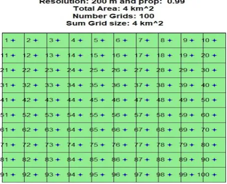
Case 2 corresponds to an optimization problem proposed in [14]. The characteristics and dimensions of the wind farm referred to in this subsection are used in the following subsubsections where the variants corresponding to Case 2: Case 2(a), Case 2(b) and Case 2(c) are solved. At the start of each subsubsection the pertinent changes in the input variables or parameters are described. The wind farm considered in the variants of Case 2 consists of a total area of 2km x 2km, which is divided into 100 squares, each with a resolution of 200m x 200m, as shown in Figure 22. Figure 23 corresponds to the wind rose, which shows the direction and speed at which the wind considered in the variants of Case 2 is propagated. These cases consider an incident wind with a uniform direction at 0° (North-South) and a constant speed of 12 m/s.
Figure 22. Characteristics and dimensions of the wind farm
Figure 23. Wind rose used for the variants of Case 2
Case 2(a)
Using the input values included in Table 8 and the wind farm data given in the previous subsection, this variant of Case 2 is optimized. Notice that the parameters corresponding to standard run number 64 shown in Table 4 are given in Table 8. To get a higher quality solution for this instance we decide to use a mutation rate of 0.006 instead of 0.01. This is because the experiment has found that the smaller the mutation rate is, the better the solutions the algorithm finds.
Table 8. Input values for Case 2(a)
Input variable Value
n (Number of turbines to be installed) 30
SurfaceRoughness(meters) 0.3
Rotor Radius(meters) 40
fcrR(value for grid spacing) 5
RotorHeight(meters) 60
referenceHeight(meters) 60
iteration 100
Proportionality 0.99
mutr(Mutation rate) 0.006
vdirspe(wind speed and direction) data.in(12
m/s at 0°)
topograp “FALSE”
elitism “TRUE”
nelit 7
selstate “FIX”
crossPart1 “RAN”
608
Abelardo Buentello-Duque
1, ETJ Volume 4 Issue 05 May 2019
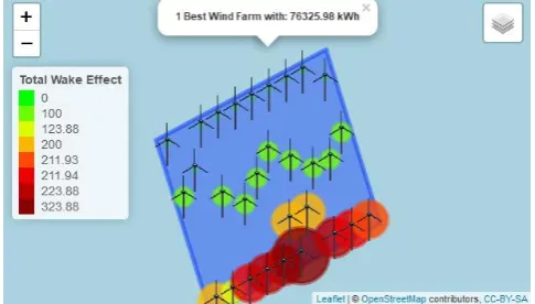
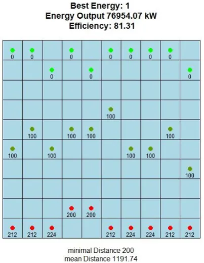
Therefore, the use of a mutation rate of 0.006 isproposed, observing that this mutation rate effectively makes the algorithm capable of exploring remote solutions in the solution space and converging on very high quality solutions. Figure 24 shows the best solution found by the algorithm for this variant of Case 2. The CPU Time that the algorithm invested in finding said solution was 204.83 seconds (3.4138 minutes of CPU), using parallel computing with 2 cores. A solution of 75605.96 kW, with an efficiency of 79.88% and a computation time of one and a half hours is reported in [14]. It is not possible to directly compare the time the algorithm took to find the solution reported in this research and the solution reported in [14], as it is not specified in [14] whether the time corresponds to the real time invested by the computer or to the CPU Time. However, if is possible to compare the quality of the solutions: the energy solution that is reported in this research is better by 720.02 units of energy in kW than the solution reported in [14], the equivalent of an 0.76% rise in efficiency. According to Figure 24, the wind turbine layout found in this research is different from the layout reported in [14].
Figure 25 shows the best solution found by the algorithm from a perspective that is closer to that of a wind farm.
Figure 26 shows the development of the wind farm’s energy efficiencies across all the generations. Said figure illustrates the evolution of efficiencies in every generation, which maintain a positive incremental trend, particularly for the maximum and average efficiencies represented by green and blue respectively. Likewise, we can see that at iteration t=90 approximately, the algorithm converges on the best solution.
Figure 24. Best solution found for the wind farm
Figure 25. Alternative representation of the best wind farm design
Figure 26. Evolution of the efficiencies throughout the generations
Case 2(b)
To optimize the second variant of Case 2 the same input values from Table 8 are used but the number of iterations are different. In this case, the algorithm is run with 300 iterations as in [14]. The reason for using 300 iterations is based, according to the premise that if the algorithm is run with a high number of iterations, this could give better solutions as the variable mutation rate would be activated more often.
Figure 27 shows the best solution found when running the algorithm for 300 iterations. The CPU time invested in finding said solution was 742.74 seconds (12.379 minutes) using computation in parallel with 2 cores. In [14] a solution of 76516.77 kW reported together with an efficiency of 80.85% when the algorithm is run for 300 iterations. According to [14], the computation time invested by the algorithm in finding said solution was 5 hours. The energy solution reported in this research exceeds the solution reported in [14] by 437.3 units of energy in kW, the equivalent of a 0.46% increase in efficiency energy. The location of wind turbines corresponding to the solution reported in [14] differs from the resulting layout reported in this research.
Figure 28 shows the best solution found from a more similar panorama to a wind farm.
609
Abelardo Buentello-Duque
1, ETJ Volume 4 Issue 05 May 2019
best solution at approximately iteration t=254, then itexplores other feasible solution spaces where it finds lower quality solutions to once again converge on the best solution between iteration t=275 and t=278.
Figure 27. Best layout of the wind farm using 300 iterations
Figure 28. Alternative representation of the solution
Figure 29. Evolution of the wind farm’s energy efficiencies per generation
Case 2(c)
This case was optimized in the same way, considering the wind farm data given in Case 2 and the input values given in Table 8, except for the rotor radius value and the fcrR value. Therefore, a rotor radius of 20m is considered in this optimization for all the turbines together with an fcrR value of 10.
Figure 30 shows the best solution found by the algorithm for this variant of Case 2. The CPU Time that the algorithm invested in finding the solution shown in Figure 30 was 287.64 seconds (4.794 minutes of CPU), using parallel computing with 2 cores. Likewise, this case is solved in [14] using turbines with a rotor radius of 20m and afcrR value of 10. Therefore, [14] reports a solution of 21585.1 kW with 91.23% efficiency. The computation time that was invested to obtain said solution is not reported. The energy solution that is reported in this research is 11.96 units of energy in kW higher than the solution reported in [14], which is the equivalent of a 0.05% increase in efficiency energy. According to Figure 30, the wind turbine layout found in this research differs from the layout reported in [14].
Figure 31 shows the evolution of the energy efficiencies corresponding to the optimization of this case. Likewise, we can see in said figure that an incremental trend of the efficiencies is maintained as the algorithm advances in the generations; however it is possible to note that, in some iterations, particularly after the iteration t=80, the algorithm finds lower quality solutions to once again converge on the best solution that had already been found.
610
Abelardo Buentello-Duque
1, ETJ Volume 4 Issue 05 May 2019
Figure 31. Evolution of the wind farm efficiencies per generation
IV.
CONCLUSIONSIn this article, the authors give a general overview of the growing worldwide importance of wind power over the last few years, together with the main factors, such as the wake effect, that affect the optimal exploitation of the power produced in a wind farm. The purpose of this research was to tackle the wind farm optimization problem, which has become an extremely important and scientifically relevant topic. The relevance of this problem within the scientific community lies in the difficulty involved with solving this problem in practice, as repeatedly physically distributing a set of wind turbines on a wind farm is hugely complex and expensive. Wind farm designers often resort to a not very efficient layout as they do not take the energy deficits caused by the wake effect into account. This results in them not being able to achieve their main objective, which is to produce the maximum amount of energy possible through the exploitation of the wind resource, starting from a particular number of wind turbines and the dimensions of the available land. It is obvious that the energy production can be significantly increased if the phenomena of the wake effects among the wind turbines is reduced as much as possible and this is only possible if they design a suitable layout of wind turbines on a wind farm. This is why we proposed the use of a Genetic Algorithm that would, in a reasonable computation time, provide good quality solutions for different wind farm scenarios that are solved in this paper. The Jensen model, which models the wake effect and calculates the energy losses caused by said phenomena when two or more turbines are located close to each other and in an incident wind direction, is also considered in the algorithm.
According to the Experiment Design carried out and the results of the cases solved in this paper, we have shown that the algorithm is capable of finding high quality solutions with little computational effort and this has an impact on two important aspects: the first is that it provides very good solutions and the second is that the energy resource the computer requires to find these solutions is relatively low. Likewise, the results presented in this paper represent better solutions in comparison to the solutions reported in [14]. The same thing happened with the computation time. The
algorithm was capable of finding better solutions, owing to the fact that first a design of experiments was done using the Case 1 scenario for the purpose of identifying those parameter values that gave the wind farm the highest possible amount of energy. Once these parameter values have been obtained, we decide to use them to find the design of another instance with 100 possible locations and 30 wind turbines, such as the variants of case 2. Using said values for the variants in Case 2 we found that the algorithm effectively found very high quality solutions with a small investment of CPU Time. The values of the parameters that are recommended for optimizing instances of large-scale wind farms are given in Table 9. It is worth mentioning that the number of iterations recommended for running the algorithm is 100, however this number could be increased if the user has enough computer resources and means or if they want to find a better solution. Despite the fact that the increased number of iterations do not guarantee the best solution being found, it does increase the probability of finding one.
Table 9. Recommended values for the key Genetic Algorithm parameters
Parameter Crossover
method
Selecti on metho d
Eliti sm
Mutation rate
No. of iteration
Value RAN FIX TR
UE
0.006 100
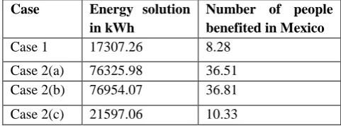
For a more realistic interpretation of the supply capacity represented by the electric power produced in a wind farm, see Table 10. Said table makes a supply analysis according to the energy solution found in each case that has been solved in this research. This analysis is based on information provided by the International Energy Agency (IEA) [18]. The IEA declares that, in 2014, the average power consumption per person in Mexico was 2090.17 kWh.
Table 10. Analysis of electric power supply in Mexico as per the solution for each case
Case Energy solution
in kWh
Number of people benefited in Mexico
Case 1 17307.26 8.28
Case 2(a) 76325.98 36.51 Case 2(b) 76954.07 36.81
Case 2(c) 21597.06 10.33
611
Abelardo Buentello-Duque
1, ETJ Volume 4 Issue 05 May 2019
applies to the basic domestic electricity utility per kWhconsumed in Mexico in the month of November 2018 is considered for the analysis. The applicable tariff, according to [19], is 0.793 MXN/kWh. Therefore, according to the
analysis, the solutions reported in this research are more attractive for electric power producers as they offer higher earnings.
Table 11. Monetary analysis
Case Energy solution reported in this paper (kWh)
Energy solution reported in the literature (kWh)
Utility that provides the solution of this paper (MXN/kWh)
Utility that provides the solution of the literature (MXN/kWh)
Difference of utility (MXN/kWh)
Case 2(a) 76325.98 75605.96 60526.50 59955.52 570.98
Case 2(b) 76954.07 76516.77 61024.57 60677.79 346.78
Case 2(c) 21597.06 21585.1 17126.46 17116.98 9.48
It must be pointed out that the main goal of this research is to promote environmental sustainability through the optimal exploitation of renewable resources, like wind, which has become one of the resources that is most likely to replace fossil fuels in the production in the future. The consumption of energy that is produced by renewable energies such as wind power implies a considerable reduction in the use of fossil fuels, which are extremely contaminating and unsustainable.
Lastly, the code of the algorithm in R of the “windfarmGA” package used in this research was developed by [14] and is available for downloading at [15]. Therefore, in [15], researchers or users in general can go there to download the package and optimize real wind farms. Said package can be used as a refining tool to get better initial wind farm layout scenarios or wind farms designed on the basis of layout principles and rules recommended by expert designers or by others empirical design methods. It can also be used as an optimization tool for finding the best layout for a certain number of wind turbines to be installed in a wind farm with irregular shape.
REFERENCES
1. Fischetti, M., &Monaci, M. 2016. Proximity search heuristics for wind farm optimal layout. Journal of
Heuristics, 22(4): 459-474. DOI:
10.1007/s10732-015-9283-4
2. Samorani, M. 2013. The Wind Farm Layout Optimization Problem. In: Pappu V (ed)
Handbook of Wind Power Systems, volume
1.Springer, Berlin, Heidelberg, pp. 21–38, ISBN:978-3-642-41080-2
3. Kusiak, A., & Song, Z. 2010. Design of wind farm layout for maximum wind energy capture.
Renewable energy, 35(3): 685-694. DOI:
10.1016/j.renene.2009.08.019
4. Shakoor, R.; Hassan, M.Y.; Raheem, A.; Wu, Y.K. 2016. Wake effect modeling: A review of wind farm layout optimization using Jensen’s model.
Renewable and Sustainable Energy Reviews, 58,
1048-1059; DOI: 10.1016/j.rser.2015.12.229
5. Horowitz, E.; Sahni, S. 1978. Fundamentals of
computer algorithms. WH Freeman & Co. New
York, NY, USA, pp. 626, ISBN: 978-0716780458 6. Archer, R., Nates, G., Donovan, S., &Waterer, H.
2011. Wind turbine interference in a wind farm layout optimization mixed integer linear programming model. Wind Engineering, 35(2): 165-175. DOI: 10.1260/0309-524X.35.2.165 7. Goldberg, D. E., & Holland, J. H. 1988. Genetic
algorithms and machine learning. Machine learning, 3(2): 95-99.
8. Holland, J. H. (1992). Adaptation in natural and artificial systems: an introductory analysis with applications to biology, control, and artificial intelligence. MIT press. Cambridge, MA, USA, pp. 232. ISBN: 978-0262581110
9. Barthelmie, R. J., Hansen, K., Frandsen, S. T., Rathmann, O., Schepers, J. G., Schlez, W., ...&Chaviaropoulos, P. K. 2009. Modelling and measuring flow and wind turbine wakes in large wind farms offshore. Wind Energy: An
International Journal for Progress and
Applications in Wind Power Conversion
Technology, 12(5), 431-444. DOI: 10.1002/we.348
10. Méchali, M., Barthelmie, R., Frandsen, S., Jensen, L., &Réthoré, P. E. 2006. Wake effects at Horns Rev and their influence on energy production. In
European wind energy conference and exhibition,
vol. 1, pp. 10-20, Athens, Greece, 27 February - 2 March 2006.
11. American Wind Energy Association. https://www.awea.org/ .Accessed on 15 May 2018. 12. Lackner, M. A., &Elkinton, C. N. 2007. An
analytical framework for offshore wind farm layout optimization. Wind Engineering, 31(1): 17-31. DOI: 10.1260/030952407780811401
13. Ainslie, J. F. 1988. Calculating the flowfield in the wake of wind turbines. Journal of Wind
Engineering and Industrial Aerodynamics, 27(1-3):
213-224. DOI: 10.1016/0167-6105(88)90037-2 14. Gatscha, S. 2016. Generic Optimization of a Wind
612
Abelardo Buentello-Duque
1, ETJ Volume 4 Issue 05 May 2019
thesis). University of Natural Resources and LifeScience, Vienna.
15. CRAN. https://cran.r-project.org/ .Accessed on 26 May 2018.
16. GEATbx: The Genetic and Evolutionary Algorithm Toolbox for Matlab. http://www.geatbx.com/ .Accessed on 08 November 2018.
17. Taha, H. A. 2010. Operations Research: An
Introduction. Pearson Education. Upper Saddle
River, New Jersey, USA, pp. 832. ISBN: 978-0132555937
18. International Energy Agency.
https://www.iea.org/statistics/statisticssearch/ .Accessed on 29 October 2018.
19. Federal Electricity Commission.