Vol. 8, No. 1, 2014, 57-63
ISSN: 2279-087X (P), 2279-0888(online) Published on 26 October 2014
www.researchmathsci.org
57
Annals of
Connectivity Analysis of a Network by Levels
Sunil Mathew1 and Jicy N2Department of Mathematics, National Institute of Technology, Calicut- 673601, India.
1
Email: [email protected], 2Email: [email protected] Received 24 September 2014; accepted 25 October 2014
Abstract. In a weighted graph model, the reduction of flow value between some pairs of nodes is more relevant and more frequent than the total disruption of the flow or the disconnection of the entire network. So it is necessary to analyse connectivity by levels. Some new connectivity and acyclicity parameters are introduced in this paper and weighted trees are categorized depending on the structure of the level graphs.
Keywords: weighted graph, partial cutnode, strength reducing set
AMS Mathematics Subject Classifications (2010): 05C22, 05C38, 05C40
1. Introduction
We can consider a totally weighted graph (Both nodes and arcs are given weights) G as a pair (σ,µ) where σ :V → ℜ and
µ
:
V
×
V
→
ℜ
. Also we denote the underlying graph by G:(σ*,µ*), where σ*={
u∈V,σ(u)>0}
andµ
* {( , )= u v ∈ ×V V;( , )u v 0}
µ
> [11]. If we have a weighted graph representing some cities and roads connecting them, thenµ
may be taken as the populations function andσ
the daily exchange of population between the cities. In such a model, connectivity plays a crucial role. Similar problems arise in all types of networks like communication, computer, biological, etc. Depending on the strength of a vertex (population, size, capacity), we can have different categories of vertices (A Class city, Big dam, etc). Also depending on the rate of flow (data flow, transport, etc.) between two nodes, we can have different categories of arcs (Broad band, national highway, etc.). Producing a path between any two nodes guarantee the connectedness of a network. But in any network, the analysis by different levels is very important. For example, high exchange of people between two big cities, less flow rate of data in a network of large capacity, etc. Also it is relevant to verify whether nodes of a given level are connected by roads of sufficient higher level. If higher category nodes are connected only by law category arcs or vice versa, the design is likely to be defective.Sunil Mathewand Jicy N
58
concept introduced in this article also generalizes the classic connectivity concepts. Some related works can be seen in [7,8,9].
A weighted graph G is a graph in which every arc e is assigned a nonnegative number w(e), called the weight of e. A graph is said to be totally weighted if both its node set and arc set are weighted [8]. The set of all the neighbours of a node v in G is denoted by NG(v) or simply N(v), and its cardinality by dG(v) or d(v)[4]. The weighted degree of v is
defined as
∑
∈ =
) (
). , ( )
(
v N x w
G v w v x
d When no confusion occurs, we denote dGw(v)
bydw(v). The weight of a cycle is defined as the sum of the weights of its arcs. An unweighted graph can be regarded as a weighted graph in which every arc e is assigned weight w(e) = 1. Thus, in an unweighted graph, dw(v) = d(v) for every node v, and the weight of a cycle is simply the length of the cycle. An optimal cycle is a cycle which has maximum weight [1].
The strength of a path P of n edges ei, for 1≤i≤n,denoted by s(P ) is equal to s(P )
= min1≤i≤n{w(ei)} [8]. The strength of connectedness of a pair of verticesu,v∈V(G), denoted by CONNG(u, v), is defined as CONNG(u, v) = {Max s(P ); P is a u -v path in G}. If u and v are in different components of G, then CONNG(u, v) = 0. A u-v path in a weighted graph G is called a strongest u-v path if s(P ) = CONNG(u, v). An edge (x, y) is
strong if its weight is at least equal to the strength of connectedness between x and y in G. [8] A connected weighted graph is called a partial tree if G has a spanning sub graph F (V; E) which is a tree, where for all arcs (x,y) of G which are not in F , we have CONNG(x, y) > µ(x, y).
Let G:(σ,µ) be a weighted graph, then for any two nodes u and v of G, the
θ
− evaluation of u and v is defined asθ
(u, v) = {α
;α
∈ℜ}, where α is the strength of astrong cycle passing through both u and v [14]. Max {
α
;α
∈θ
( , ); , ∈σ
*} v u vu is defi-
ned as the cycle connectivity between u and v in G and is denoted by Cu,vG. Cycle connectivity of a graph G is defined as CC(G) = max{C , ;u,v∈
σ
*}G v
u .
2. t-cuts and connectedness levels
Consider a totally weighted graph G:(σ,µ), For t∈ℜ,the direct t-cut of G or t-cut of
G, denoted by Gtor (
σ
t,µ
t) is the sub graph of G with node set} ) ( /
{x V x t
t = ∈
σ
≥σ
and arc setµ
t ={(x,y)∈V×V/µ
(x,y)≥t}. Consider Example 1.Even though both the structures in figure 2 are the same, the connectivity of G2 is
more than that of G1. The strength of a path in G2 is 8 where as that of G1 is 1. Now
consider another example (Figure 3).
All t-cuts Gtof G1 in (Figure 3) are connected for t∈(4,8], but not in G2. Thus
G1 shows some kind of connectedness which is not in G2. Motivated by the above
examples, we have the following definition.
59
}. ,
, / ) , ( min{
)
(G CONN x y x y V x y
C = G ∈ ≠
Example 1. (Figure 1)
5 5 5
3 1 3 3
3 2 3 2 2 3 2
G G2 G3
Figure 1: t-cuts of a graph
Now consider the following two graphs.
7 9
7 8
1 9
G1 G2
Figure 2: Different connectivity levels.
G1 G2 Figure 3: Connected t-cuts.
Sunil Mathewand Jicy N
60 connected.
Definition 2. Let G be a weighted graph. Then G is called weakly connected if there
exists some t-cut of G which is connected.
In the previous example, G1 is weakly connected. Clearly every connected weighted
graph G is weakly connected. But converse is not true. (G1 in previous example is weakly
connected but not connected.)
Given a graph G, the cyclomatic number of G is defined as m- n + p where n, m and p denote the number of vertices, number of edges and number of connected components respectively. Using this we have a new definition as follows.
Definition 3. [9] Let G be a weighted graph with n vertices, m edges and p connected
components. The cyclomatic function
ψ
(G,t):ℜ→N∪{0},t∈ℜis defined by) , (G t
ψ
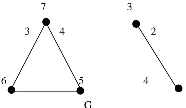
= cyclomatic number of Gt = mt −nt + pt,where nt, mt, pt denotes the number of vertices strong edges and connected components of Gt.Example 2: Consider the following weighted graph (Figure 4) with two components, 5
vertices and 5 edges.
7 3
3 4 2
6 5 5 4
G
Figure 4: Cyclomatic number of a disconnected graph
Here for any t∈(−∞,2), h(G,t)=mt −nt + pt =4−5+2=1. For t =2.1,
. , 1 3 5 3 ) 1 . 2 ,
(G etc
h = − + =
Now we shall discuss some of the elementary properties of the cyclomatic function
), , (G t
ψ
First we have a trivial proposition.Proposition 1. For any totally weighted graph G, and t∈ℜ,
ψ
(G,t)≥0..Also note that h is a piecewise constant function with finitely many jumps. In the next theorem, we show that ψ is a non increasing function.
Theorem 1. Let G be a totally weighted graph and let t, t'∈ℜ such that t≥t'. Then
). , ( ) ,
( '
t G t
G
ψ
61
Proof: We have mt ≤mtIimplies m m k1
I
t t = −
, k1∈Ζ and k1 ≥0. Also
I
t t
n
n ≤
implies mt =mtI −k2, k2∈Ζ and k2 ≥0. The number of connected components of t
G may increase, decrease or remains same as t ranges over ℜ. Thus for t≥t',
3
k p
pt = tI − , for some k3∈ℜ and k3 ≥0.
Thus (G,t) (m k1)
I
t − =
ψ
-(n k2)I
t −
+ (ptI −k3)
=
ψ
(G,tI )+(k2 −k1 −k3)=. ) ,
(G tI +k
ψ
We shall prove that k > 0 is impossible. If k2 <0 there is nothing toprove. So we prove the following cases.
Case 1. k2 =0.
This case implies that the vertex set does not change from Gt to GtI. Thus k3 ≤0,
because components cannot decrease by edge suppression. Thus −k3 ≤k1, which implies k≤0.
Case 2. k2 >0.
We denote h, the number of eliminated connected components of GtI.. Obviously
h
k3 ≤ and k2 ≤h . Let h=k2 −s; s∈{0,1,2,...,k2}. From the definition of s,
s
k1≥ and thus k=k2 −k3 −k1 ≤k2 −k3 +s−k, which implies k≤s−k1≤0.
Next we have a definition.
Definition 4. The cyclomatic kernel of a weighted graph G is defined as }. 0 ) , ( ; { )
(G = t∈ℜ G t =
Ka
ψ
In other words, Ka(G) is the set of all real numbers such that Gt is a forest. In the previous example, 5∈Ka(G). Using this kernel, we have a measure for the acyclic
nature of the graph.
Definition 5. The strong acyclic level of a weighted graph G is defined as )}
( ;
inf{ )
(G t t K G
Sw = ∈ a and which is same as the cycle connectivity of the weighted
graph G. i.e. Sw(G)=CC(G). It will help to measure the number of strong cycles in a
given graph G.
The following theorem can be easily proved from the above definition and by using the properties of cycle connectivity.
Theorem 3. Let G:(σ,µ) be a weighted graph, then Gt has no cycles if and only if
Sunil Mathewand Jicy N
62
Proof: Let G:(σ,µ) be a connected weighted graph such that Gt has no cycles in it. Let CC(G) be the cycle connectivity of G such that Cu;vG < t for every u,v∈V. For otherwise suppose that there exist a cycle in G, whose strength is more than or equal to t. which will be remain in Gt. which is a contradiction. Conversely, suppose CC(G) be the cycle connectivity of G such that CC(G) < t, to prove Gt has no cycles. Assume that Gt has a cycle (say) C. Then strength of the cycle C(s(C)) is more than or equal to t, therefore CC(G)≥s(C)≥t, again a contradiction. This completes the proof.
Now we can introduce a definition using cycle connectivity.
Definition 6. A weighted graph G:(σ,µ) is said to be fully strong acyclic if and only if CC(G)=0.
Clearly a weighted graph is fully acyclic if and only if it is a partial forest. Let G1, G2, …, Gn be the components of G, then for each Gi, i= 1,2,…,n is a partial tree. Then
by the theorem 2.7 in [15], CC(G)=0.
Definition 7. A weighted graph G:(σ,µ) is strong acyclic by t-cuts if there exist a ℜ
∈
t such that Gt has no cycles.
Proposition 2. Every strongly acyclic graph is strong acyclic by t- cuts.
Proof: Let G:(σ,µ) be any strongly acyclic weighted graph, then CC(G) = 0 and hence Cu,v
G
= 0 for every pair of nodes in G. That is G will be strong acyclic by t-cuts.
3. Concluding remarks
Connectivity concepts are the key in graph clustering and network problems. The classical parameters are dealing with the disconnection of the graph. In practical applications the reduction in the flow is more frequent than the disconnection. The authors made an attempt to generalize the connectivity concepts in weighted graphs. Also one of the major theorems in Graph theory due to Whitney is generalized.
REFERENCES
1. Dhanyamol M V and Sunil Mathew, Distance in weighted graphs, Annals of Pure and Applied Mathematics, 8(1) (2014) 79-87.
2. G.A.Dirac, Some theorems on abstract graphs, Proc. London Math. Soc., (3) 2(1952) 69 - 81.
3. J.A.Bondy and G.Fan, Optimal paths and cycles in weighted graphs, Ann.Discrete Mathematics, 41(1989) 53-69.
4. J.A.Bondy and G.Fan, Cycles in weighted graphs, Combinatorica, 11(1991) 191-205. 5. J.A.Bondy, H.J.Broersma, J.van den Heuvel and H.J.Veldman, Heavy cycles in
weighted graphs, Discuss. Math. Graph Theory, 22 (2002) 7-15.
6. R.Diestel, Graph Theory, Graduate Texts in Mathematics, Second edition, 173, Springer, 2000.
63
8. M.Pal, Intersection graphs: An introduction, Annals of Pure and Applied Mathematics, 4(2013) 43-91.
9. Sunil Mathew and M S Sunitha, Anjali N, Some connectivity concepts in bipolar fuzzy graphs, Annals of Pure and Applied Mathematics, 7(2) (2014) 98-108.
10. Sunil Mathew and M.S.Sunitha, Types of arcs in a fuzzy graph, Information Sciences, 179 (11) (2009) 1760-1768.
11. Sunil Mathew and M.S.Sunitha, On totally weighted interconnection networks, Journal of Interconnection Networks, 14(1) (2013) 1-16.
12. Sunil Mathew and M.S.Sunitha, Some connectivity concepts in weighted graphs, Advances and Applications in Discrete Mathematics, 6 (1) (2010) 45-54.
13. Sunil Mathew and M.S.Sunitha, Bonds in graphs and fuzzy graphs, Advances in Fuzzy Sets and Systems, 6(2) (2010) 107-119.
14. Sunil Mathew and M.S.Sunitha, Cycle connectivity in weighted graphs, Proyecciones Journal of Mathematics, 30 (1) (2011) 1-17.
15. Sunil Mathew and M.S.Sunitha, Cycle connectivity in fuzzy graphs, Journal of Intelligent and Fuzzy System, 24 (2013) 549-554.