Detection of ULF Analogy Using ACO Based
Algorithm in Power Distribution Networks
Ramesh. Gamasu
Department of EEE, SACET, Cherala (A.P), India Email: [email protected]
Venkata Ramesh Babu. Jasti
Department of EEE, RISE Krishna Sai Group of Institutions, Ongole (A.P), India Email: [email protected]
Abstract—Distribution and Transmission are two key systematic parameters in power systems engineering and power systems are places a huge role in nation’s progress. Now a day’s Power Distribution Networks are exaggerated by different tribulations like voltage dip conditions, harmonics, swell and sag conditions and faults etc. Out of mentioned, faults are very dangerous that affects voltage stability and load balancing phenomenon. The proposed article will able to explain the identification of Unbalanced Load Faults (ULF) using modern optimization techniques. This technique initiates the problem by taking number of iterations and contextual procedure i.e. Ant Colony Optimization (ACO). This is best methodology apt for any mechanical and electrical distribution networks helps to negotiate the problem by taking number of iterations. The proposed article suggests how to identify the unbalanced fault analogy and faults behavior using ACO based algorithm. The overall topology was investigated and simulated and highly graphical facilities are provided with help of MAT Lab Simulation.
Index Terms—unbalanced load faults (ULF), ant colony optimization (ACO), modern optimization technique, power distribution networks, fault searching behavior
I. INTRODUCTION
A Transmission line is one of the most important prototype parameter of power system which is used to synchronizing the transmission and distribution networks. Adequately, the transmission and distribution may have the losses and voltage abrupt conditions; faults too. Faults in the transmission line places a prominent role in the power systems. Ideally, due to the fault conditions the entire system may damages. In order to the faults besides there is a voltage dip conditions and different voltage fluctuations are occurring over there. In the entire power system, the transmission and distribution are main phenomenon systems [1]. Faults are occurring due to unavoidable fluctuations in voltage and currents and short circuit condition and internal losses in synchronous generators. These may avoided by maintaining the proper node and base voltages at terminal conditions. The
Manuscript received October 29, 2013; revised May 14, 2014.
ant and food as a power system. Here the same phenomenon is applied for obtain the pre and post fault detection. This article only will explain the fault detection and identification by using multi variable approach.
II. OVER VIEW OF POWER DISTRIBUTION NETWORK -TESTING OF POWER SYSTEM MODEL
The test power system consists of two equal distant 320kV parallel lines having 50kms length. The two lines are feed from generators G1 and G2 respectively as represented in the block diagram itself. The both line models are distributed type and used for power distribution from source to user end. Manually, the lines are initiated and transposed by R, L, C parameters. They are compressed with positive and zero sequence faults. The source end was designated by a transformer and load end too. Here the fault was created in any one of the lines are creates the disturbance and telephonic interference in the lines are nothing but harmonics and are due to fault conditions [6]. The Fig. 1 Shows power distribution network model represents a source and load end with probable fault. The proposed power system model resembles the test system used for fault identification which is crested in any one of the two parallel lines itself.
Figure 1. Tested power distribution network model
III. FAULT DETECTION USING ACO IN POWER
DISTRIBUTION NETWORKS
ACO is super imposed genetic algorithm based methodology. The proposed paper describes the search the fault in power system like an ant searching for food. The proposed article explains the comparison of fault occurrence with ant’s propagation. Here the fault was compared with insect ant and the material food was compared against with test power syatem. Fig. 2 initiates the pre-fault and post-fault data identification using ACO Methodology [7].
Figure 2. Fault identification using ACO
IV. ANT COLONY OPTIMIZATION FOR FAULT
DETECTION
Ant colony optimization (ACO) is based on the cooperative behavior of real Fault colonies, which are able to find the shortest path from their nest to a Modified
source. The Fault colony optimization process can be explained by representing the optimization problem as a multilayered graph, in that Fault conditions are replaced by faults and Modified source is test system. Where the number of layers is equal to the number of design variables and the number of nodes in a particular layer is equal to the number of discrete values permitted for the corresponding design variable. Thus each node is associated with a permissible discrete value of a design variable. Fig. 3 denotes a problem with six design variables with eight permissible discrete values for each design variable, The ACO process can be explained as follows. Let the colony consist of N Faults.
Figure 3. Fault based single layer ACO network
A. Fault Searching Behavior
A Fault k, when located at node i, uses the pheromone trail τij to compute the probability of choosing j as the next node
(1)
where α denotes the degree of importance of the pheromones and Ni(K) indicates the set of neighborhood nodes of Fault k when located at objective i. Then beside of all objectives i contain all the nodes directly connected to node i accept the predecessor node (i.e., the last node visited before i). This will prevent the Fault from returning to the same node visited immediately before node i. A Fault travels from node to node until it reaches the destination (Modified) node is updated as follows
ij ij + (K) (2)
Due to the incremental changes in the proto type phenomenon, the critical nature of this arc being selected by the forthcoming Fault condition will increase.
B. Pheromone Trail Evaporation for Fault Detection
When a Fault k moves to the next node, the pheromone evaporates from all the arcs ij according to the relation
ij (1-p) ij; (i, j) A (3)
where p∈(0, 1] is a parameter and A denotes the segments or arcs traveled by Fault k in its path from home to destination. The decrease in pheromone intensity favors the exploration of different paths during the search process. This favors the elimination of poor choices made in the path selection. This also helps in bounding the maximum value attained by the critical procedure. A step is process of a complete description of Fault’s movement, pheromone evaporation and pheromone deposit. After all the Faults return to the home node (nest), the pheromone information is updated according to the relation
ij = (1-p) ij + ij (K)
(4)
where ρ∈(0, 1] is the evaporation rate (also known as the pheromone decay factor) and _τ (k) ij is the amount of pheromone deposited on arc ij by the best Fault k. The goal of pheromone update is to increase the pheromone value associated with good or promising paths [10]. The pheromone deposited on arc ij by the best Fault is taken as
ij (K)
= Q/LK (5)
where Q is a const Fault and Lk is the length of the path traveled by the kth Fault (in the case of the travel from one city to another in a traveling salesman problem). Equation (5) can be implemented as
ij (K)
= (6)
where fworst is the worst value and fbest is the best value of the objective function among the paths taken by the N Faults, and ζ is a parameter used to control the scale of the global updating of the pheromone. The larger the value of ζ, the more pheromone deposited on the global best path, and the better the exploitation ability [9]. The aim of Equation (5) is to provide a greater amount of pheromone to the tours (solutions) with better objective function values.
V. PRAPOSED ALGORITHM FOR FAULT DETECTION
The orentational procedure of ACO algorithm for solving a minimization problem can be summarized as follows
Step 1
Assume a suitable number of Faults in the colony (N). Assume a set of permissible discrete values for each of the n design variables. Denote the permissible discrete values of the design variable xi as xil, xi2, ..., xip and (i=1, 2, ..., n). Assume equal amounts of pheromone τij(1) initially along all the arcs or rays (discrete values of design variables) of the multilayered graph shown. The superscript to τij denotes the iteration number.
For simplicity, τij(1) can be assumed for all arcs ij. Set the iteration number l = 1
Step 2
(a) Compute the probability (pij) of selecting the arc or ray (or the discrete value) xij as
Pij = rij(l)/ lm(l); I=1, 2, ..., n; j=1, 2, 3, ..., p (7)
Which can be seen to be same as Equation (1) with α=1. A larger value can also be used for α.
(b) The specific path (or discrete values) chosen by the kth Fault can be determined using random numbers generated in the range (0, 1). For this, we find the cumulative probability ranges associated with different paths of Fig. 1 based on the probabilities given by Equation (7). The specific path chosen by Fault k will be determined using the roulette-wheel selection process in step 3(a).
Step 3
(a) Generate N random numbers r1, r2...rN in the range (0, 1), and one for each Fault. Determine the discrete value or path assumed by Fault k for variable i as the one for which the cumulative probability range [found in step 2(b)] includes the value ri.
(b) Repeat step 3(a) for all design variables i=1, 2...n. (c) Evaluate the objective function values corresponding to the complete paths (design vectors X(k) or values of xij chosen for all design variables as i=1, 2...n by Fault k, k=1, 2...N) is
FK = f(X(k)); k=1, 2, ..., N (8)
To obtain the better and worst paths chosen by different Faults are
Fbest = K = 1, 2, 3min..., N{ fk} (9)
Step 4
Test for the convergence of the process. The process is assumed to have converged if all N Faults take the same best path. If convergence is not achieved, assume that all the Faults return home and start again in search of Test Power System. Set the new iteration number as l = l+1, and update the pheromones on different arcs (or discrete values of design variables) as
ij(l) = ij(old)+ ij(K) (11)
where τij(old) denotes the pheromone amount of the previous iteration left beyond the convergent process, which is written as
ij(old) = (1-p) ij(l-1) (12)
and Δτij(K) is the pheromone deposited by the best Fault k on its path and the Summation extends over all the best Faults k (if multiple Faults take the same best path). Note that the best path involves only one arc ij (out of p possible arcs) for the design variable i. The evaporation rate or pheromone decay factor ρ is assumed to be in the range 0.5 to 0.8 and the pheromone deposited is Δτij(K) computed using Equation (6).
With the new values of Δτij(l), go to step 2. Steps 2, 3, and 4 are repeated until the process converges, that is, until all the Faults choose the same best path. In some cases, the iterative process is stopped after completing a pre-specified Maximum number of iterations (lmax).
VI. RESULTS AND DISCURSIONS FOR TEST SYSTEM
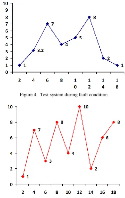
The proposed test system contains identification of pre-fault and post-faults on distribution networks. The proposed algorithm can be used for observing the most common fault in power distribution network i.e. L-G Fault. Fig. 5 Represents performance of test power system during the fault condition, initiates that fault current on y-axis and impedance on x-axis respectively. If we observe the Fig. 5 fault represents seven number of iterations are over there.
The pre-fault and post fault are observed by using ACO based algorithm. In, Fig. 5 utmost of 7 cycles are assembled are first cycle initiates starting node point of fault current i.e. pre-fault and the next sixth cycle initiates maximum probability of fault current of test system in power distribution networks.
The test system fed by unbalanced load in abnormal conditions and faults are represented with number of iterations. Each of iteration resembles the portion of fault in working conditions. The Fig. 5 represents seven number of cycles are nothing but faults. So, during unbalanced load conditions the test system able to show the more number of iteration without any optimization or additive complex technique applied over there.
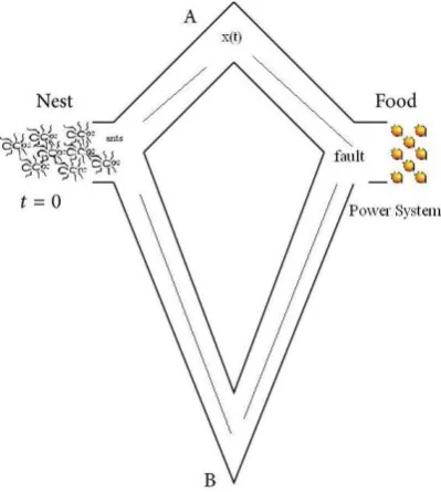
In Fig. 4, on x axis fault impedance and y-axis fault current was represented. Fig. 4 represents the performance characteristics of ACO based algorithm during unbalanced L-G fault on the distribution network during abnormal condition, having less number of iterations as compared to the performance Characteristics of Fig. 5 having without any control tool, however the
overall topology of the proposed system can only be done with ACO optimization method such that the performance characteristics shows that better performance during any un-desirable or abnormal conditions also.
Figure 4. Test system during fault condition
Figure 5. Implementation of ACO based algorithm for test system
Figure 6. Comparison of fault occurrence in test system, with and without AC optimization
better performance as compared to conventional un-control modeled characteristics.
VII. CONCLUSIONS
The paper presents pre-determination and identification of fault using Ant Colony Optimization. The proposed topology explains the most dangerous faults scenario described as an Unbalanced Load Fault Analogy. Here the fault is characterized by the insect ant, and the power system initiated as a material food itself.
The evaluated simulation are explains comparison of fault variations with source and destination of ant.
If more iteration is over there in ACO, then the power system is affected by more. If there over less, the power system affects less. The overall topology was conducted for a proposed test system. Hence the ACO based algorithm helps to find or identify the most dangerous fault scenario in PDN. The entire topology was modeled and simulated, investigated. The high graphical representations are mentioned with help of MATLAB/Simulink.
APPENDIX
TABLEI. ILLUSTRATION FOR FAULT ANALOGY USING ACOBASED ALGORITHM
S.NO
Characterization of Single Line-Ground Fault Number of Harmonic
Spectrum Fault Resistance Voltage Sag Voltage Swell
Harmonic Distortion in sequence order Rf in Ω P.U P.U in %
1 1st 0.66 0.8259 0.698 100 2 3rd 0.76 0.9867 0.7 47.22 3 5th o.86 0.8634 0.567 67.9 4 7th 0.96 0.9645 0.4 45.67 5 9th 1.06 0.9143 0.55 56.45 6 11th 1.2 0.9472 0.53 34.67 7 13th 1.8 0.9316 0.23 89.67 8 15th 2.02 0.9531 0.5744 56.33 9 17th 2.08 0.9713 0.9 63.4 10 THD 0.3 0.9241 0.22 48.3 11 Power Factor of Load 0.2 0.9376 0.89 100
REFERENCES
[1] K. S. Pandya and S. K. Joshi, “A survey of the optimal power flow methods,” Journal of Theoretical and Applied Information
Technology (JATIT), pp. 450-458, 2008.
[2] Z. F. Qiu, G. Deconnick, and R. Belmans, “A literature survey of optimal power flow problems in the electricity market context,” in
Proc. Power Systems Conference and Exposition, 2009, pp.
1845-1850.
[3] J. A. Momoh, M. E. El-Hawary, and R. Adapa, “A review of selected optimal power flow literature to 1993 part I: Non linear and quadratic programming approaches,” IEEE Transactions on
Power Systems, vol. 14, pp. 96-104, Feb. 1999.
[4] A. J. Wood and B. F. Wollenberg, Power Generation, Operation
and Control, New York: John Wiley and Sons, 1984.
[5] B. H. Chowdhury and S. Rahman, “A review of recent advances in economic dispatch,” IEEE Transactions on Power Systems, vol. 5, no. 4, pp. 1248-1259, 1990.
[6] M. Dorigo and T. Stuzel, Ant Colony Optimization, The MIT Press, 2004.
[7] A. Colorni, M. Dorigo, and V. Maniezzo, “Distributed optimization by ant colonies,” in Proceedings of the First
European Conference on Artificial Life, F. J. Varela and P.
Bourgine, Eds. Cambridge, MA: MIT Press, 1992, pp. 134-142. [8] M. Dorigo, V. Maniezzo, and A. Colorni, “The ant system
optimization by a colony of cooperating agents,” IEEE
Transactions on Systems, Man, and Cybernetics—Part B, vol. 26,
no. 1, pp. 29-41, 1996.
[9] S. Rao Singiresu, Engineering Optimization Theory and Practice, John Wiley & Sons, 2009.
[10] M. F. Meteb, “Particle swarm optimization (PSO) based optimal power flow for the Iraqi EHV network,” A thesis, University of Baghdad, 2012.
Mr. Ramesh. Gamasu was born in India, on October 15, 1989. He
obtained his B.Tech Degree in Electrical and Electronics Engineering from JNT University, Kakinada (A.P), and India in 2010. He worked as assistant professor of Electrical Science Engineering Department in Centurion University of Technology & Management, Perlakhemundi (Odisha) and Electrical Engineering Department of RISE Krishna Sai Group of Institutions, Ongole (A.P). Currently, working as Research Scholar in Department of Electrical & Electronics Engineering, St. Ann’s College of Engineering & Technology (A.P), India. He is member of various Engineering societies like IAENG, IACSIT, IACSE, ASEE, and UACEE, IAEM etc. He published various research articles and letters on Power Systems Engineering. His areas of interest include Power Systems Deregulation and reconstruction, role of artificial techniques for diagnosing the power quality problems and Power Systems Dynamics etc.
Mr. Venkata Ramesh Babu. Jasti was born in Chimakurthy, Andhra