Simultaneous allocation of reliability & redundancy using minimum total cost of ownership approach

(1)

SIMULTANEOUS ALLOCATION OF RELIABILITY &

REDUNDANCY USING MINIMUM TOTAL COST OF

OWNERSHIP APPROACH

G. Kanagaraj*

Department of Mechanical Engineering, Thiagarajar College of Engineering, Madurai, Tamil Nadu, India, 625015

N. Jawahar

Depaertment of Mechanical Engineering and Dean (R&D) Thiagarajar College of Engineering, Madurai, Tamil Nadu, India, 625015

Received: 17/7/2011 Accepted: 29/8/2011 Online: 11/9/2011

ABSTRACT

This paper addresses the mixed integer reliability redundancy allocation problems to determine simultaneous allocation of optimal reliability and redundancy level of components based on three objective goals. System engineering principles suggest that the best design is the design that maximizes the system operational effectiveness and at the same time minimizes the total cost of ownership (TCO). To evaluate the performance of the TCO allocation numerical experiments were conducted and compared with previous for the series system, the series-parallel system, the complex (bridge) system and the over speed protection system. From the results of the numerical investigation, reliability redundancy allocation based on minimum TCO will lead to a more reliable, economical design for the manufacturer as well as user compared with the initial cost optimum design and conventional reliability optimum design.

KEYWORDS:Reliability and redundancy allocation, Mixed integer non-linear programming, Total cost of ownership

NOMENCLATURE

b Upper limit on resource

&V The upper limit on the cost of the system FL The cost of each component in subsystemL &L Cost function of subsystemL

DTC Down Time Cost JL The ithconstraint function

Q The number of subsystem or stages in the system N Number of failures over the mission time ofW. PC Procurement Cost

r ≡(UUU,….rQ), the vector of the component reliabilities for the system RC Replacement Cost

UL The reliability of each component in subsystemL

(2)

-&$50( *̖.DQDJDUDMHWDO 9RO1R6HSW 5L Reliability function of subsystemL

5V The system reliability t Design life of the system TCO Total Cost of Ownership

9V The upper limit on the sum of the subsystems products of volume & weight YL The volume of each component in subsystemL

:V The upper limit on the weight of the system ZL The weight of each component in subsystemL

x ≡([[[,…..[Q), the vector of the redundancy allocation for the system [L The number of components in subsystemL

βi Factor for replacement of components of subsystemL γ Annual down time cost

INTRODUCTION

In general, designers concentrate to reduce the procurement cost of the system or product to as low as possible to be more competitive in the market, because the price is a widely used determinant for the customer in the selection of product. This criterion often results in poor customer satisfaction. The reason is that the costs to be incurred in the years after purchase may be significant, exceeding initial procurement cost. Due to the highly volatile and competitive nature of the global market, customers (or) users today are closely examining the long term cost of ownership of a system instead of looking only at the lowest procurement cost. Hence, such costs should be included in any purchase decisions. The total cost of ownership (TCO) is a purchasing tool and philosophy to understand the true cost of buying a particular good or service [1].Gartner’s definition[2] of TCO states that TCO consists of the costs incurred throughout the lifecycle of an asset, including acquisition, deployment, operation, support and retirement. TCO models were initially developed by Gartner Research in 1987 and are now widely accepted. Carr and Ittner [3] present an overview of TCO approaches used by several organizations. Handfield and Pannesi [4] explored the concept of TCO specifically for components, using the product life cycle approach.

The system engineering principles suggest that the best design is the design that maximizes the system operational effectiveness and at the same time minimizes the TCO. The strength of TCO is to provide and understand the future costs that may not be apparent when an item is initially purchased [1-5]. TCO can be applied to the government (federal, state, local), industries (automobile, rail industry, semi conductor industry, aerospace, airlines, electronics, information etc.,) and individual business [6-9]. TCO provides many benefits that are documented in the literature [10] and confirmed by case studies. TCO drives the customer to look beyond the initial procurement cost for decision making, and provides a meaningful way to integrate reliability and maintenance strategies with product sales and service offerings [11]. Based on the above considerations, this paper addresses TCO based design strategy to evolve a product or system configuration that corresponds to a minimum TCO in order to provide maximum satisfaction to the customers.

One of the most important cost drivers in the TCO equation is product reliability and it will significantly impact maintenance costs, as well as fixed costs such as downtime [11]. The major cost elements of TCO are: Procurement Cost, Replacement Cost and Down Time Cost. Fig. (1) shows the relationship between the costs of TCO and system reliability.

Cost versus reliability curve for a system exhibits the following features:

 Procurement cost is a monotonic increasing function of reliability

 Replacement cost is a monotonically decreasing function of reliability

 Downtime cost is a monotonically decreasing function of reliability

Let5be the reliability of the system that corresponds to minimum TCO. However, the functional or

(3)

correspond to5V and the optimal reliability becomes5V. On the other hand 5V≥ R(Refer 5in Fig.

(1)), minimum TCO would correspond to 5 and the optimal reliability becomes 5. The above discussions reveal that system reliability 5Vinfluences TCO. Besides, for a multistage series system

having redundant components at all stages, the system reliability5Vdepends on stage reliability5L

i.e.,

5

_V



I

5

_L

(1)

Suppose each stage‘i’is built with[Lnumber of components, then5L is a function of its component

reliabilityULand number of redundant components‘xL’:

i.e,

5

_L



I

(

U

_L

,

[

_L

)

(2)

The arguments describe that the TCO of the system, thus becomes a function ofUL[L( for allL) which

can be stated as:

)

,

(

U

_L

[

_L

I

7&2



(3)

The cost elements of TCO are: Procurement Cost (PC), Replacement Cost (RC), and Down Time Cost (DTC) defined as a function ofUL [Las:

) , ( 1

) , (

1 ln

) , (

1 1

1



 F [ 5 [ U W

U [ 5 U

[

& Q

L L L L L

L L Q

L L L L Q

L L L L 

 

  _  

   

  

   

  







 



TCO (4)

The first term in the above TCO equation represents the total procurement cost of the system. The second term represents the replacement cost of failure components during the system life time. Failure of all components in any stageL leads to system failure. At that instance, all the components in the stage are replaced with new components. The cost of replacing the components in‘i’is considered as

L FL Where L is the factor to account for the increase in component cost and labor cost that is

incurreds during replacements. Suppose the failure time of components at stageL,1[_LQ, follows a

negative exponential distribution with failure rate λi and the system is required to operate for a

specified time t. Then the reliability of stageLis 5_L HLW H1 _{where N = number of failures over the}

R1 R0 R2

Reliability of the system Rs Total Cost of Ownership (TCO)

Procurement Cost

Down time Cost

Replacement Cost

C

o

st

TCOR2

TCOR1

TCORo

(4)

-&$50( *.DQDJDUDMHWDO 9RO1R6HSW

mission time ofW. Therefore the number of times, each component‘i’with ‘[L’number of components

in parallel fails during the system life time‘t’ becomes:

Ni 

  

  

    

  

  

U OQ

L

[ L

1 1

1 ₍₅₎

Hence the cost of replacement of failure component is stated as:

1 2

RC

1 1

1

  

   

  

   

 

  



 L L L L

Q

L L [

[ F

U OQ

L  

(6)

The last term in TCO equation represents the downtime cost to the user since the system is not available for productive work during the failure and replacement time. Therefore, TCO of the system is influenced by the component reliability (UL) and the redundancy level ([L). The mathematical

formulation of TCO pertains to the well-known reliability redundancy allocation problem (RRAP) belonging to the class of nonlinear mixed integer programming problems with separable constraints. The mathematical formulation becomes a mixed integer nonlinear programming problem (MINLP) in which the continuous variables represent the component reliabilities and the integer variables represent the level of redundancy. RRAP is the hardest problem in the reliability optimization field because the decision variables are mixed-integer and the system reliability function is nonlinear, non-separable, and non convex [12]. Reliability apportionment encompasses the problem of assigning the correct reliability to each subsystem in such a manner that the overall system reliability is equal to its goal. Once these subsystem reliabilities are established, the designer can select the materials, configurations, and types so that the overall reliability requirement can be achieved.

This paper attempts to evolve a system, based on minimum total cost of ownership approach in order to provide maximum satisfaction to the customers. The number of components[Land the component

reliability ULof subsystemLare the decision variables to be determined for three different conflicting

goals namely maximization of system reliability, minimization of system cost, and minimization of system total cost of ownership. The problem template is expressed as:

Q L HJHU LQW SRVLWLYH [

U

J WR VXEMHFW

I 0LQ RU 0D[

L

L    



 

1 b

x r,

x r

1 0

(7)

WhereULand[Lare the reliability and the number of components in theLWKsubsystem respectively;f (•)

is the objective function to be maximized or minimized; andg (•)is the constraint function and b is the upper limit on the resource;Qis the number of subsystems.

The structure of this paper is organized as follows: In the first section the problem statement and corresponding mathematical equations are addressed for the three objective goals. The next section presents some numerical examples and results are presented to compare the performance of TCO based allocation with traditional allocation methods. Final section concludes with some important remarks.

PROBLEM STATEMENT

(5)

Case 1. Maximization of system reliability (R. based allocation)

n

i

eger

int

positive

x

r

)

(

g

to

subject

)

,

(

f

R

Max

imize R

max

which

&

Find

i i s s









1 b

x

r,

x

r

x

r

1

0

(8)

Case 2. Minimization of system cost (C based allocation)

n

i

eger

int

positive

x

r

)

(

g

to

subject

)

(

f

C

Min

imize C

min

which

&

Find

i i s s









1 b

x

r,

x

r,

x

r

1

0

(9)

Case 3. Minimization of total cost of ownership (TCO based allocation)

n i eger int positive x r ) ( g to subject ) ( f TCO Min imize TCO min which & Find i

i    

   1 b x r, x r, x r 1 0 (10)

Where r is the reliability vector (r1,r2,…..rn) of the system and x is the redundancy vector

(x1,x2,……xn) of the system respectively;f (•)is the objective function to be maximized or minimized;

and g (•) is the constraint function and b is the upper limit on the resource; n is the number of subsystems. The goal is to determine the number of the component (

x

_i) and the component reliability (

r

_i) in each subsystem to achieve optimal objective values.

NUMERICAL EXAMPLES AND DISCUSSION

To evaluate the performance of the proposed TCO based allocation approach from traditional reliability allocation approaches, four mixed integer nonlinear reliability design problems (P1~P4) are solved. These examples are the series system, series-parallel system, complex (bridge) system and overspeed protection system. All the above problems are solved separately in three cases. The mathematical formulations of the four reliability-redundancy problems are furnished below.

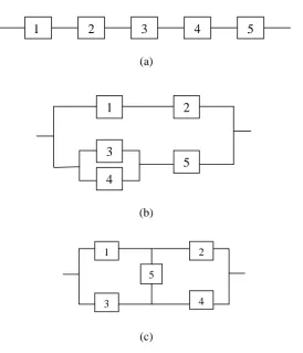
P1. SERIES SYSTEM [Fig. (2(a))]

Case 1. Maximization of system reliability (R based allocation)

Max f( ) R_i(x_i) n i



  1 x r, (11) Subject to: s n i i i i s n i i i i i s n i i

i x V r x x C w x x W

v 



 i  







 

1 1 1

(6)

JCARME G.Kanagaraj, et al. Vol. 1, No. 1, Sept. 2011

n

i

x

r

_i



_i





1 positive

integer,

1

0

] ) 4 / exp( [ ) ln / 1000 ( C 1 s



    n i i i i

i r x x

Min



i ₍₁₂₎

Subject to s i i n i R x R 



 ) ( 1 , _s n i i i i s n i i

i x V w x x W

v 









1 1

2 )] 4 / exp( * [ , *

n

i

x

r

_i



_i





1 positive

integer,

1

0

Min





1



1-(1- )



) -1 ( -1 1 ln ] ) 4 / exp( [ ) ln / 1000 ( TCO 1 1 1     t r x c r x x r n i x i i i i n i x i n i i i i i i i i                          





   (13) Subject to: s n i x i R

r i 

 



1 ) 1 ( 1

( , _s

n

i

i x V

v 



1

2

* , _s

n

i

i i

i x x W

w 



1 )] 4 / exp( * [

n

i

x

r

_i



_i





1 positive

integer,

1

0

P2. SERIES-PARALLEL SYSTEM [Fig. (2(b))]

Max

f

(

r

,

x

)



1 

(

1 

R

₁

R

₂

)(

1 

(

1 

R

₃

)(

1 

R

₄

)

R

₅

)

(14)

Subject to s n i i i i s n i i i i i s n i i

i*x V , ( /lnr ) [x exp(x / )] C , w [x *exp(x / )] W

v 



 i  







 

1 1 1

2 4 4 1000 



n

i

x

r

_i



_i





1 positive

integer,

1

0

] ) 4 / exp( [ ) ln / 1000 ( C 1 s



    n i i i i

i r x x

Min



i ₍₁₅₎

Subject to s

R

)

R

)

R

)(

R

(

)(

R

(







1

₁ ₂

1

₃

1

₄ ₅

1

, _s

n i i i i s n i i

i*x V , w [x *exp(x / )] W

v 







 1 1

2

4

n

i

x

r

_i



_i





1 positive

integer,

1

(7)

Min TCO ln 1  c x



R



t

R )] / x exp( x [

c _i _i _i _s

n i s n i i i

i   

              



  1 4 1 1 (16) Subject to: s

R

)

R

)

R

)(

R

(

)(

R

(







1

₁ ₂

1

₃

1

₄ ₅

1

, _s

n i i i i s n i i

i*x V , w[x *exp(x / )] W

v 







 1 1

2

4

n

i

x

r

_i



_i





1 positive

integer,

1

0

P3. COMPLEX (BRIDGE) SYSTEM [Fig. (2(c))]

5 4 3 2 1 5 4 3 2 5 4 3 1 5 4 2 1 5 3 2 1 4 3 2 1 5 3 2 5 4 1 4 3 2 1

2 R

R

)

(

f

Max









x

r,

(17) Subject to s n i i i i s n i i i i i s n i i

i*x V , ( /lnr ) [x exp(x / )] C , w [x *exp(x / )] W

v 



 i  







 

1 1 1

2 4 4 1000 



n

i

x

r

_i



_i





1 positive

integer,

1

0

] ) 4 / exp( [ ) ln / 1000 ( C 1 s



    n i i i i

i r x x

Min



i ₍₁₈₎

Subject to s

R









5 4 3 2 1 5 4 3 2 5 4 3 1 5 4 2 1 5 3 2 1 4 3 2 1 5 3 2 5 4 1 4 3 2 1

2

s n i i i i s n i i

i x V w x x W

v 









1 1

2 )] 4 / exp( * [ , *

n

i

x

r

_i



_i





1 positive

integer,

1

0

Min TCO ln 1  c x



R



t

R )] / x exp( x [

c _i _i _i _s

n i s n i i i

i   

              



  1 4 1 1 (19) Subject to s

R









5 4 3 2 1 5 4 3 2 5 4 3 1 5 4 2 1 5 3 2 1 4 3 2 1 5 3 2 5 4 1 4 3 2 1

2

s n i i i i s n i i

i x V w x x W

v 









1 1

2 )] 4 / exp( * [ , *

n

i

x

r

_i



_i





1 positive

integer,

1

(8)

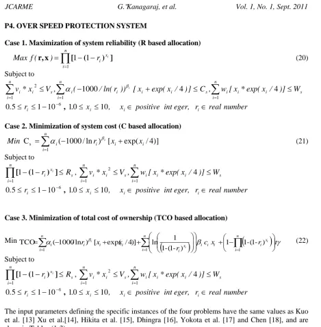
P4. OVER SPEED PROTECTION SYSTEM



    n i x i i r ) ( f Max 1 1

1 ( ) ]

[ x r, (20) Subject to s n i i i i s n i i i i i s n i i

i*x V , ( /ln(r )) [x exp(x / )] C , w [x *exp(x / )] W

v 



 i  







 

1 1 1

2 4 4 1000 



number real r eger, int positive x , x . r

.  i   ,  i  i i 

 10 0 1 10 1 5 0 6

] ) 4 / exp( [ ) ln / 1000 ( C 1 s



    n i i i i

i r x x

Min



i ₍₂₁₎

Subject to s n i x i R

r i 

 



1

1

1 ( ) ]

[ , _s

n i i i i s n i i

i*x V , w [x *exp(x / )] W

v 







 1 1

2 4 number real r eger, int positive x , x . r

.  i   ,  i  i i 

 10 0 1 10 1 5 0 6

Min





1



1-(1- )



) -1 ( -1 1 ln ] ) 4 / exp( [ ) ln / 1000 ( TCO 1 1 1     t r x c r x x r n i x i i i i n i x i n i i i i i i i i       _                   





   (22) Subject to s n i x i R

r i 

 



1

1

1 ( ) ]

[ , _s

n i i i i s n i i

i*x V , w [x *exp(x / )] W

v 







 1 1

2 4 number real r eger, int positive x , x . r

.5 _i 110 , 10 _i 10 _i _i 

0 6

The input parameters defining the specific instances of the four problems have the same values as Kuo et al. [13] Xu et al.[14], Hikita et al. [15], Dhingra [16], Yokota et al. [17] and Chen [18], and are show in Tables (1-3).

(9)

(a)

(b)

(c)

Fig. 2. (a) Series system, (b) series-parallel system and (c) complex (bridge) system.

For measuring the improvement, MPI (maximum possible improvement) can be used to measure the amount of improvement of the solutions found by the proposed approach to the previous best known solutions [20]. MPI is the fraction that the best feasible solution achieved of the maximum possible improvement, it is described as:

) 1

(

) (

(%)

_ _ _

other s

other s TCO s

R R R

MPI

  

Where Rs_TCOrepresents the system reliability obtained by the proposed minimum TCO approach and

Rs_otherrepresents the system reliability obtained by other approaches in literature. By using the index,

it is shown that the proposed TCO based allocation made more improvement in P2 ~ P4.

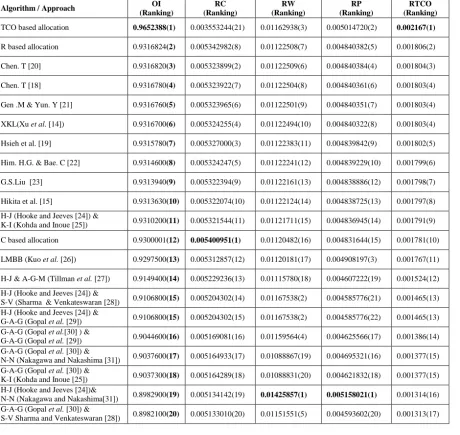
Based on the results of Table (5), five performance criteria for further comparison between this proposed method of allocation and other 20 combination approaches are defined as follows:

1) Optimality index (OI): the optimal system reliability value. 2) Reliability-cost ratio (RC): the ratio of system reliability to cost

3) Reliability-weight ratio (RW): the ratio of system reliability to the used weight

4) Reliability-product ratio (RP): the ratio of system reliability to the weight and volume of used product

5) Reliability-total cost of ownership (RTCO): the ratio of system reliability to the total cost of ownership.

1

2

3

4

5

1

2

3

5

4

1 2

3 4

(10)

Table 1. Data used in series system (P1) and complex system (P3).

i 105_α

i βi wivi2 wi V C W

1 2.330 1.5 1 7

110 175 200 2 1.450 1.5 2 8

3 0.541 1.5 3 8

4 8.050 1.5 4 6

5 1.950 1.5 2 9

Table 2. Data used in series - parallel system (P2).

i 105_α

1 2.500 1.5 2 3.5

180 175 100 2 1.450 1.5 4 4.0

3 0.541 1.5 5 4.0

4 0.541 1.5 8 3.5

5 2.100 1.5 4 4.5

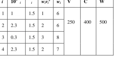
Table 3. Data used in overspeed protection system (P4).

i 105_α

1 1 1.5 1 6

250 400 500 2 2.3 1.5 2 6

3 0.3 1.5 3 8

4 2.3 1.5 2 7

(11)

Table 4. Comparison of solutions obtained with other algorithms for series system (P1).

Hikita et al.[15]

Kuo et al. [13]

Xu et al. [14]

Hsieh et al. [19]

Chen [18] Chen [20] R based allocation

C based allocation

TCO based allocation

x (3,2,2,3,3) (3,2,2,3,3) (3,2,2,3,3) (3,2,2,3,3) (3,2,2,3,3) (3,2,2,3,3) (3,2,2,3,3) (3,2,2,3,3) (3,2,2,3,3)

r

0.777143 0.77960 0.77939 0.779427 0.779266 0.779435 0.7793989 0.7774428 0.8270626

0.867514 0.80065 0.87183 0.869482 0.872513 0.871805 0.8718370 0.8703728 0.9063120

0.896696 0.90227 0.90288 0.902674 0.902634 0.902824 0.9028854 0.9017688 0.9291183

0.717739 0.71044 0.71139 0.714038 0.710648 0.711503 0.7114025 0.7088759 0.7732283

0.793889 0.85947 0.78779 0.786896 0.788406 0.787720 0.7877995 0.7859155 0.8336877

Rs 0.931363 0.92975 0.931677 0.931578 0.931678 0.931682 0.9316824 0.9300001 0.9652388

MPI (%) 49.4% 50.5% 49.1% 49.1% 49.1% 49.11% 49.1% 50.3%

Slacks of (g1~ g3)

27 27 27 27 27 27 27 27 27

0.00000 0.000010 0.013773 0.121454 0.001559 0.625102 -0.000008 2.80809 -96.65

7.518918 10.57248 7.518918 7.518918 7.518918 7.518918 7.518918 7.518918 7.518918

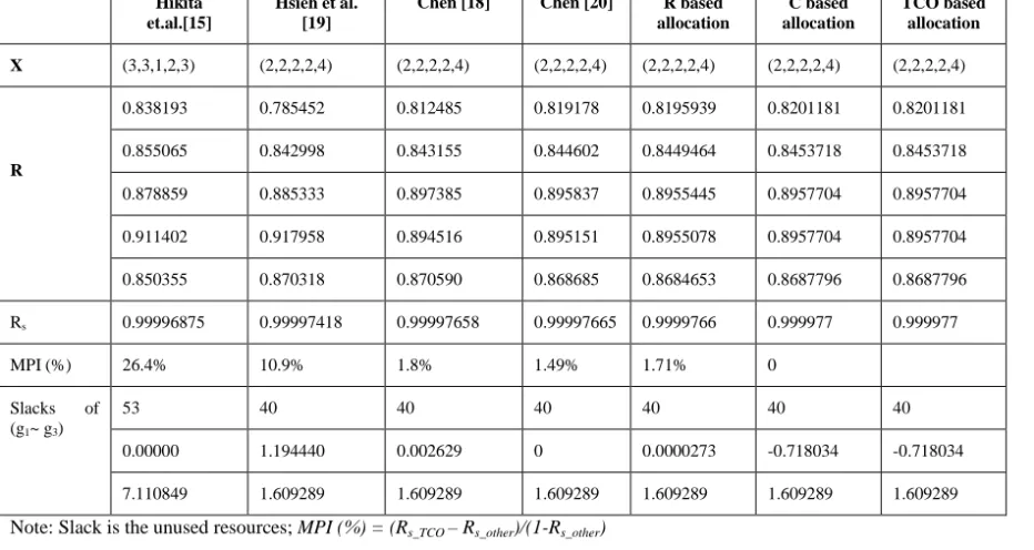
Note: Slack is the unused resources; MPI (%) = (Rs_TCO–Rs_other)/(1-Rs_other)

Table 5. Comparison of solutions obtained with other algorithms for series–parallel system (P2).

Hikita et.al.[15]

Hsieh et al. [19]

TCO based allocation

X (3,3,1,2,3) (2,2,2,2,4) (2,2,2,2,4) (2,2,2,2,4) (2,2,2,2,4) (2,2,2,2,4) (2,2,2,2,4)

R

0.838193 0.785452 0.812485 0.819178 0.8195939 0.8201181 0.8201181

0.855065 0.842998 0.843155 0.844602 0.8449464 0.8453718 0.8453718

0.878859 0.885333 0.897385 0.895837 0.8955445 0.8957704 0.8957704

0.911402 0.917958 0.894516 0.895151 0.8955078 0.8957704 0.8957704

0.850355 0.870318 0.870590 0.868685 0.8684653 0.8687796 0.8687796

Rs 0.99996875 0.99997418 0.99997658 0.99997665 0.9999766 0.999977 0.999977

MPI (%) 26.4% 10.9% 1.8% 1.49% 1.71% 0

Slacks of (g1~ g3)

53 40 40 40 40 40 40

0.00000 1.194440 0.002629 0 0.0000273 -0.718034 -0.718034

7.110849 1.609289 1.609289 1.609289 1.609289 1.609289 1.609289

(12)

Table 6.Comparison of solutions obtainedwith other algorithms for complex system (P3).

Hikita et.al. [15]

Hsieh et al. [19]

Gen &Yun [21]

TCO based allocation

X (3,3,2,3,2) (3,3,3,3,1) (3,3,3,3,1) (3,3,3,3,1) (3,3,3,3,1) (3,3,2,4,1) (3,3,3,3,1) (3,3,2,4,1)

R

0.814483 0.814090 0.808258 0.812485 0.815878 0.8280840 0.7454456 0.8280864

0.821383 0.864614 0.866742 0.867661 0.868265 0.8578051 0.8084230 0.8578048

0.896151 0.890291 0.861513 0.861221 0.859217 0.9142417 0.7928609 0.9142407

0.713091 0.701190 0.716608 0.713852 0.711529 0.6481475 0.5929169 0.6481462

0.814091 0.734731 0.766894 0.756699 0.752922 0.7041650 0.6709976 0.7041618

Rs 0.99978937 0.99987916 0.999889 0.9998892 0.9998893 0.9998896 0.9989999 0.9998896

MPI (%) 47.58% 8.63% 0.54% 0.35% 0.23% 0 88.96%

Slacks of (g1~ g3)

18 18 18 18 18 5 18 5

1.854075 0.376347 0.001494 0 -0.00002 79.5119 0

4.264770 4.264770 4.264770 4.264770 4.264770 1.56047 4.2647 1.56047

Note: Slack is the unused resources; MPI (%) = (Rs_TCO–Rs_other)/(1-Rs_other)

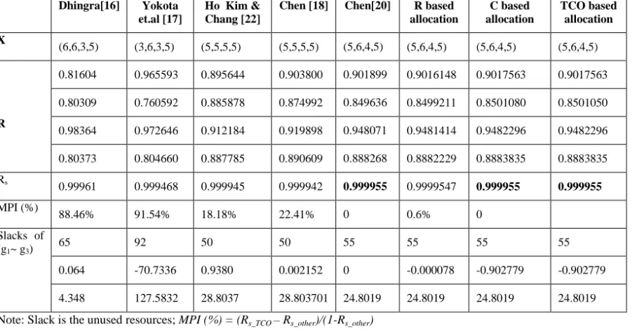
Table 7.Comparison of solutions obtainedwith other algorithms for overspeed system (P4).

Dhingra[16] Yokota et.al [17]

Ho Kim & Chang [22]

Chen [18] Chen[20] R based allocation

TCO based allocation X

(6,6,3,5) (3,6,3,5) (5,5,5,5) (5,5,5,5) (5,6,4,5) (5,6,4,5) (5,6,4,5) (5,6,4,5)

R

0.81604 0.965593 0.895644 0.903800 0.901899 0.9016148 0.9017563 0.9017563

0.80309 0.760592 0.885878 0.874992 0.849636 0.8499211 0.8501080 0.8501050

0.98364 0.972646 0.912184 0.919898 0.948071 0.9481414 0.9482296 0.9482296

0.80373 0.804660 0.887785 0.890609 0.888268 0.8882229 0.8883835 0.8883835

Rs

0.99961 0.999468 0.999945 0.999942 0.999955 0.9999547 0.999955 0.999955 MPI (%)

88.46% 91.54% 18.18% 22.41% 0 0.6% 0

Slacks of

(g1~ g3) 65 92 50 50 55 55 55 55

0.064 -70.7336 0.9380 0.002152 0 -0.000078 -0.902779 -0.902779

4.348 127.5832 28.8037 28.803701 24.8019 24.8019 24.8019 24.8019

(13)

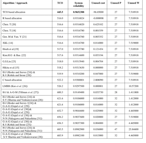
Table 8. Comparison of results of example 1.

Algorithm / Approach TCO System

reliability

Unused cost Unused P Unused W

TCO based allocation 445.5 0.9652388 -96.65000 27 7.518918

R based allocation 516.0 0.9316824 -0.000008 27 7.518918

Chen. T [20] 516.6 0.9316820 0.625102 27 7.518918

Chen. T [18] 516.6 0.9316780 0.001559 27 7.518918

Gen .M & Yun. Y [21] 516.6 0.9316760 0.003352 27 7.518918

XKL [14] 516.6 0.9316700 0.014000 27 7.519000

Hsieh et al.[19] 517.0 0.9315780 0.121454 27 7.518918

Kim.H.G & Bae. [22] 517.6 0.9314600 0.053194 27 7.518918

G.S.Liu [23] 518.0 0.9313940 0.004704 27 7.518918

Hikita et al [15] 518.2 0.9313630 0.000000 27 7.518918

H-J (Hooke and Jeeves [24]) &

K-I (Kohda and Inoue [28]) 519.9 0.9310200 0.047000 27 7.519000

C based allocation 522.2 0.9300001 2.808090 27 7.518918

LMBB (Kuo et al. [26]) 526.2 0.9297500 0.000001 27 10.57200

H-J & A-G-M (Tillman et al. [27]) 600.3 0.9149400 0.033730 28 1.411800

S-V (Sharma and Venkateswaran [28]) 621.6 0.9106800 0.014000 32 1.412000 H-J (Hooke and Jeeves 1[24]) &

G-A-G (Gopal et al. [29]) 621.6 0.9106800 0.014000 32 1.412000 G-A-G (Gopal et al. [30])&

G-A-G (Gopal et al. [29]) 652.7 0.9044600 0.025000 32 4.465000 G-A-G (Gopal et al. [30]) &

N-N (Nakagawa and Nakashima [31]) 656.2 0.9037600 0.020000 27 7.519000 G-A-G (Gopal et al. [30]) &

K-I (Kohda and Inoue [25]) 656.3 0.9037300 0.004000 27 4.465000 H-J (Hooke and Jeeves [24]) &

N-N (Nakagawa and Nakashima [31]) 683.5 0.8982900 0.036000 47 25.84600 G-A-G (Gopal et al. [30])&

(14)

Table 9. Detailed comparisons of results for example 1.

Algorithm / Approach OI (Ranking)

RC (Ranking)

RW (Ranking)

RP (Ranking)

RTCO (Ranking) TCO based allocation 0.9652388(1) 0.003553244(21) 0.01162938(3) 0.005014720(2) 0.002167(1)

R based allocation 0.9316824(2) 0.005342982(8) 0.01122508(7) 0.004840382(5) 0.001806(2)

Chen. T [20] 0.9316820(3) 0.005323899(2) 0.01122509(6) 0.004840384(4) 0.001804(3)

Chen. T [18] 0.9316780(4) 0.005323922(7) 0.01122504(8) 0.004840361(6) 0.001803(4)

Gen .M & Yun. Y [21] 0.9316760(5) 0.005323965(6) 0.01122501(9) 0.004840351(7) 0.001803(4)

XKL(Xu et al. [14]) 0.9316700(6) 0.005324255(4) 0.01122494(10) 0.004840322(8) 0.001803(4)

Hsieh et al. [19] 0.9315780(7) 0.005327000(3) 0.01122383(11) 0.004839842(9) 0.001802(5)

Him. H.G. & Bae. C [22] 0.9314600(8) 0.005324247(5) 0.01122241(12) 0.004839229(10) 0.001799(6)

G.S.Liu [23] 0.9313940(9) 0.005322394(9) 0.01122161(13) 0.004838886(12) 0.001798(7)

Hikita et al. [15] 0.9313630(10) 0.005322074(10) 0.01122124(14) 0.004838725(13) 0.001797(8)

K-I (Kohda and Inoue [25]) 0.9310200(11) 0.005321544(11) 0.01121711(15) 0.004836945(14) 0.001791(9)

C based allocation 0.9300001(12) 0.005400951(1) 0.01120482(16) 0.004831644(15) 0.001781(10)

LMBB (Kuo et al. [26]) 0.9297500(13) 0.005312857(12) 0.01120181(17) 0.004908197(3) 0.001767(11)

H-J & A-G-M (Tillman et al. [27]) 0.9149400(14) 0.005229236(13) 0.01115780(18) 0.004607222(19) 0.001524(12)

S-V (Sharma & Venkateswaran [28]) 0.9106800(15) 0.005204302(14) 0.01167538(2) 0.004585776(21) 0.001465(13) H-J (Hooke and Jeeves [24]) &

G-A-G (Gopal et al. [29]) 0.9106800(15) 0.005204302(15) 0.01167538(2) 0.004585776(22) 0.001465(13) G-A-G (Gopal et al.[30] ) &

G-A-G (Gopal et al. [29]) 0.9044600(16) 0.005169081(16) 0.01159564(4) 0.004625566(17) 0.001386(14) G-A-G (Gopal et al. [30]) &

N-N (Nakagawa and Nakashima [31]) 0.9037600(17) 0.005164933(17) 0.01088867(19) 0.004695321(16) 0.001377(15) G-A-G (Gopal et al. [30]) &

K-I (Kohda and Inoue [25]) 0.9037300(18) 0.005164289(18) 0.01088831(20) 0.004621832(18) 0.001377(15) H-J (Hooke and Jeeves [24])&

N-N (Nakagawa and Nakashima[31]) 0.8982900(19) 0.005134142(19) 0.01425857(1) 0.005158021(1) 0.001314(16) G-A-G (Gopal et al. [30]) &

S-V Sharma and Venkateswaran [28]) 0.8982100(20) 0.005133010(20) 0.01151551(5) 0.004593602(20) 0.001313(17)

CONCLUSIONS

(15)

not only for designing a system for high reliability applications but for minimum cost of ownership to the user.

ACKNOWLEDGEMENTS

The authors thank the management of the Thiagarajar College of Engineering, Madurai, for the facilities provided to carry out this work. The authors are very much thankful to anonymous referees for their valuable suggestions and comments that helped us make this paper more valuable.

REFERENCES

[1] L. M.Ellram “The total cost of ownership: an analysis approach for purchasing”, International

Journal of Physical Distribution & Logistics Management, Vol. 25, No. 8, pp. 4-23, (1995) .

[2] W. B. Gartner “A framework for describing the phenomenon of new venture creation”

Academy of Management Review, Vol. 10, pp 696-706, (1985).

[3] L. P. Carr and C. D.Ittner “Measuring the Cost of Ownership”, Journal of Cost Management, Vol. 6, No. 3, pp. 7-13. (1992).

[4] R. Handfield and R. Pannesi “Managing component life cycles in dynamic technological

environments”Journal of Purchasing and Materials Management, Spring pp. 20-27, (1994).

[5] L. M Ellram. and A.B. Maltz “The use of total cost of ownership concepts to model the

outsourcing decision”, International Journal of Logistics Management, Vol. 6, No. 2, pp. 4-23, (1995).

[6] P. N. Pasqua “Power supply procurement, defining the value of your supplier, Total cost of ownership”Applied Power Electronics Conference and Exposition, 1996, APEC’96 Conference

Proceedings, Vol.1, pp. 47-54, (1996).

[7] E. F. Hitt, Battelle and O. H. Columbus,“Total ownership cost use in management”, Digital Avionics Systems Conference, Proceedings., 17th DASC. The AIAA/IEEE/SAE, Vol. 1, A32-1-5,

(1998).

[8] Sohn and Moon.“How important is reliability in a Total cost of ownership analysis of Clusters” Techwise Research, Inc November 1999 Version 1.1 [email protected].

[9] S. Castellani and A. Grasso O'Neill J., Tolmie P. “Total cost of ownership: issues around

reducing cost of support in a manufacturing organization case”, E-Commerce Technology Workshops, pp. 122–130, (2005).

[10] L. M. Ellram “A frame work of total cost of ownership”, International Journal of Logistics Management, Vol. 4, No. 2, pp. 49-60, (1993).

[11] E. R. Carrubba “Integrating life-cycle cost and cost-of-ownership in the commercial sector” Reliability and Maintainability Symposium, 1992. Proceedings. Annual, 21-23 Jan., pp

101-108, (1992).

[12] C. Ha and W. Kuo“Multi-Path Approach for Reliability-Redundancy allocation using a scaling

method”,Journal of Heuristics, Vol. 11, No. 3, pp. 201-217, (2005).

[13] W. Kuo, C. L. Hwang and F. A. Tillman “A note on heuristic methods in optimal system

reliability”,IEEE Transactions on Reliability, R 27, pp.320-324, (1978).

[14] Z. Xu, W. Kuo and H. H. Lin “Optimization limits in improving system reliability”, IEEE Transactions on Reliability, Vol. R-39, pp.51-60, (1990).

[15] M. Hikita, Y. Nakagawa and H.Narihisa “Reliability optimization of systems by a surrogate

-constraints algorithm”,IEEE Transactions on Reliability, Vol. 41,No. 3, Pp. 473-80,(1992).

[16] A. K. Dhingra “Optimal apportionment of reliability & redundancy in series systems under

multiple objectives”,IEEE Transactions on Reliability, Vol. 41, No. 4, Pp.576-582, (1992).

[17] T. Yokota, M. Gen and Y. X.Li “Genetic algorithm for nonlinear mixed-integer programming

problems and its application”,Computers and Industrial Engineering, Vol. 30, No. 4, pp.

(16)

[18] T. C. Chen “IAs based approach for reliability redundancy allocation problems”, Applied Mathematics and Computation, Vol. 182, pp. 1556-1567, (2006).

[19] Y. C. Hsieh, T. C Chen and D. L Bricker “Genetic algorithms for reliability design problems”, Microelectronics Reliability, Vol. 38, No. 10, pp. 1599-1605, (1998).

[20] T. C. Chen “Penalty Guided PSOfor reliability design problems”, PRICAI 2006, LNAI 4099,

pp. 777-786, (2006).

[21] M. Gen and Y. Yun “Soft computing approach for reliability optimization”, Reliability

Engineering & System Safety, Vol. 91, pp.1008-1026, (2006).

[22] K. Ho-Gyun and B. Chang-Ok “Reliability-redundancy optimization using simulated annealing

algorithms”, Journal of Quality in Maintenance Engineering, Vol. 12, No. 4, pp. 354-363,

(2006).

[23] G. S. Liu “A combination method for reliability-redundancy optimization”, Engineering

Optimization, Vol. 38, No. 4, pp. 485-499, (2006).

[24] R. Hooke and T. A. Jeeves “Direct search solution of numerical and statistical problems”,

Journal of the Association of Computing Machinery, Vol. 8, No. 2, pp. 212-229, (1961).

[25] T. Kohda and K. Inoue “A reliability optimization method for complex system with the criterion local optimality”, IEEE Transactions on Reliability, Vol. R-31, Apr, pp. 109-111, (1982).

[26] W. Kuo, H. H. Lin, Z. Xu and W.Zhang “Reliability optimization with the Lagrange-multiplier and branch-and-bound technique”, IEEE Transactions on Reliability, Vol. 36, No. 5,

pp.624-630, (1987).

[27] F. A Tillman, C. L Hwang and W.Kuo “Determining component reliability and redundancy for

optimum system reliability, IEEE Transaction on Reliability, R 26, No. 3, pp.162-165, (1977). [28] J. Sharma and K. V. Venkateswaran“A direct method for maximizing the system reliability”.

IEEE Transactions on Reliability R-20: pp 256–9, (1971).

[29] K. Gopal and K. K. Aggarwal “A new method for solving reliability optimization problem, IEEE Transaction on Reliability, R 28, pp.36-38, (1978).

[30] K. Gopal, K. K. Aggarwal and J.S. Gupta“A new method for solving reliability optimization problem”, IEEE Transactions on Reliability, Vol. R-29, Jan, pp 36-38, (1980).