doi: 10.11648/j.ajtas.20130203.12
Using the Markov Chain Monte Carlo method to make
inferences on items of data contaminated by missing
values
I. Karangwa, D. Kotze
Department of Statistics and Population Studies, University of the Western Cape, Cape Town, South Africa
Email address:
[email protected] (I. Karangwa), [email protected] (D. Kotze)
To cite this article:
I. Karangwa, D. Kotze. Using the Markov Chain Monte Carlo Method to Make Inferences on Items of Data Contaminated by Missing Values, American Journal of Theoretical and Applied Statistics. Vol. 2, No. 3, 2013, pp.48-53. doi: 10.11648/j.ajtas.20130203.12
Abstract:
The Markov Chain Monte Carlo (MCMC) is a method that is used to estimate parameters of interest under difficult conditions such as missing data or when underlying distributions do not fit the assumptions of Maximum Likelihood processes. The objective of this process is to find a probability distribution known as a posterior distribution in Bayesian analysis that can be used to estimate target parameters. In this paper, we consider a case where data are contaminated with missing values and therefore need to be adequately handled using missing data techniques before making inferences on them. A review of the mathematics involved in MCMC procedures in the presence of missing data is presented. Furthermore, we use real data to compare inferences made using multiple imputation based on the multivariate normal model (MVN) that uses the MCMC procedure, the case deletion (CD) missing data method that discards subjects with missing values from the analysis, and the fully conditional specification (FCS) multiple imputation method that uses a sequence of regression models to fill in missing values. Assuming that data are missing completely at random (MCAR) on continuous and normally dis-tributed variables, the following findings are obtained: (1) The higher the proportion of missing data on a variable of interest, the more the relationship between that variable and the dependent variable is distorted when all missing data methods are applied. (2) Multiple imputation based methods produce similar estimates which are better than estimates from the case deletion method. (3) At some stage (when the proportion of missing data becomes high), none of the missing data techniques can help to maintain an initially existing relationship between the dependent variable and some of the covariates of interest in the dataset.Keywords:
Markov Chain Monte Carlo (MCMC), Missing Data, Missing Completely At Random (MCAR), Multiple Imputation, Multivariate Normal Model (MVN), Fully Conditional Specification (FCS)1. Introduction
Missing data are common and a major problem in dif-ferent fields of research [6, 9, 16]. It is not given much at-tention by some researchers especially those who are not methodologists or statistical experts. This is due mainly to the lack of familiarity with the existing statistical literature on missing values or the ignorance of the impact that miss-ing data can have on statistical inferences [13]. A traditional way of dealing with missing data is to eliminate these ob-servations from the analysis, a strategy that is referred to as the Case Deletion or Listwise Deletion (CD) method. Dis-carding missing observations from analysis reduces the sample size, which leads to a sample that is not representa-tive of the population. Consequently, the power of the
would have been obtained if we had complete data [14]. This paper focuses mainly on the data augmentation me-thod based on a multivariate normal model (MVN) that uses the Markov Chain Monte Carlo procedure. It assumes a normal distribution for the variables in the imputation model [14].
A number of studies compared this method to the fully conditional specification (FCS) method which is also a multiple imputation-based method that uses a sequence of regression models to impute missing values, depending on the nature of the variables to be imputed; linear regression for continuous variables, logistic regression for binary va-riables, multinomial regression for polytomous vava-riables, etc. [10, 17, 19]. These studies concentrated on different aspects and applied the two methods to data with a mixture of variables (continuous, discrete and semi-continuous). Mixed results were obtained; some concluded that the MVN was better than the FCS [17, 19] and others found the opposite [1, 10]. Van Buuren [17] also highlighted that the two methods are identical when applied to continuous and normally distributed data. In this paper, we use different simulated data sets to also give our view of these two me-thods in terms of their performance when data are missing completely at random (MCAR) on continuous and normal-ly distributed variables.
2. Markov Chain Monte Carlo Methods
in the Presence of Missing Values in a
Dataset
When data are missing, the primary objective of a re-searcher is to generate unbiased estimates in order to make good inferences. This is not generally easy when available data (observed data after discarding missing items) are used. With MCMC methods, the available data need to be aug-mented with simulated values of the missing data in order to get good parameter estimates. The procedure is as fol-lows.
Let Y be multivariate data from a normal distribution,
(
Y|θ)
=N( )
β,Σp , where θ denotes the unknown model parameters such as regression coefficients βand covariance matrix
Σ
. In the presence of missing values we have(
Yobs Ymis)
Y = , , where
Y
obsandY
mis represent the observedand missing parts respectively. Missing values in
Y
mis are drawn from the distribution of missing data given the ob-served data,p(
Ymis|Yobs)
. However, this distribution isdif-ficult to sample from directly because it depends on the posterior distribution of the unknown parameters θ ,
(
Yobs)
pθ| . Initially, the data augmentation (DA) method was designed to approximate this distribution when data are incomplete [14]. The observed data need to be augmented with unobserved data
Y
mis such that the conditionaldis-tribution p
(
Ymis|Yobs)
becomes easier to sample from. To illustrate the above, consider the posterior distribution(
Yobs)
pθ| . When data are incomplete, this distribution can be written in terms of an integral as follows:
(
Yobs)
p(
YobsYmis) (
pYmis Yobs)
dYmis pθ
| =∫
θ
| , | (1)To evaluate this density, the Monte Carlo method can be used. That is independent copies of Ymis(Ymis(1),Ymis(2), …, Ymis(n)) can be drawn from the conditional distribution p(Ymis | Yobs) and then the average
( )
( )
∑
p Y jn |
1 θ
can be computed and serve as an approxima-tion of p(Yobs), where Y (j) denotes the augmented dataset (Yobs,Ymis,(j)) for j = 1, 2,..., n and Ymis(j) = (Ymis)1(j), (Ymis)2(j), …, (Ymis)n(j).
In the Markov Chain Monte Carlo context, the above mentioned idea can be simply implemented using the Im-putation-Parameter (IP) algorithm suggested by Schafer [14] which works as follows. Assuming a multivariate normally distributed data, at the tth iteration one needs to draw
Y
mis(t+1)from ( | , (t)) obs mis Y Y
p θ , and then draw θ(t+1) from
)
,
|
(
Y
obsY
mis(t+1)p
θ
. The former step is referred to as the Imputation (I) step and the latter as the Parameter (P) step. The resulting sequence forms a Markov chain{
(1) (1)}{
(2) (2)} {
( 1) ( 1)}
, ,..., , ,, mis mist+ t+
mis Y Y
Y
θ
θ
θ
which mustcon-verge to the distribution p
(
Ymis|Yobs,θ
)
[3, 7, 8] and usedin the Multiple Imputation to estimate parameters when data
are missing. In words, in the I-step missing values
Y
misare simulated for each observation independently by using the observed data Yobs and the estimates of the mean vector and covariance matrix represented by θ(t). The P-step uses thecomplete data set (full data with generated missing values) from the I-step to generate new estimates of the mean vector and covariance matrix, which are to be used in the next I-step to simulate new values. The repetition of these two steps (I-step and P-step) creates a Markov chain (sequence of random variables in which the distribution of each ele-ment is related to the values of the previous one). Their role is to generate a distribution of values from which random samples of simulated missing values are obtained and used in Multiple Imputation methods to estimate parameters when data are missing. The chain needs to be long enough for the distribution of the elements to stabilize to a common distribution referred to as the stationary distribution [14].
3. Methodology
3.1. Description of the Original Data Set
eco-nomic data. The sample of women in the analysis includes women of reproductive age who were not pregnant at the time of interview and who were sexually active. Respon-dents were asked about their knowledge and use of contra-ception methods, etc. Information on whether they have ever used contraception was first obtained and then the types of contraception methods used were asked. Contra-ception methods used included the modern (i.e. pill, injec-tions and other), traditional (i.e. abstinence and other) and folkloric (i.e. herbal plant and other) methods. The depen-dent variable considered for the analysis was the women's contraceptive use status measured as any contraceptive method use by including all women who reported using modern, traditional and folkloric methods coded as 1 and 0 to represent women who have never used any contraceptive method. The purpose was to determine whether and to what extent certain covariates such as the age and education in years of a woman, her marital status, etc., are associated with the woman's use of contraception. Thus, slopes, stan-dard errors and results of hypothesis tests were considered as outcomes of interest to be analyzed.
3.2. Simulation of Data Sets with Missing Values
In order to assess the performance of the Multiple Impu-tation using the Markov Chain Monte Carlo method or MVN and other methods (case deletion and fully condi-tional specification), datasets were created with some of their values missing completely at random (MCAR) on variables age and education that were statistically signifi-cant in the regression model. This assumption means that missingness probabilities are not related at all to any other variables in the data set.
As an application, eight data sets were created with dif-ferent rates of missingness; 5%, 10%, 15%, 20%, 25%, 30%, 35% and 40% on variables age and education. Based on the variables of interest (age and education) with no missing data, a 0 - 1 random generator if the observation was missing (1) or not (0) was constructed. This means that missing data are random draws from the Bernouilli distribution with the parameter p that represents the percentage of missing values of interest (percentages of missingness in this case). Tech-nically, this can be represented as follows. Let Yi be a
com-plete data vector for respondent i. Then Yi can be partitioned
into Yi,obs and Yi,mis, the observed and missing parts
respec-tively. That is, Yi = (Yi,obs,Yi,mis). Let also Ri = (rij) be the
missing data indicator, where rij = 1 if a value is missing and
rij = 0 otherwise. Given some parameter
θ
, the MCARas-sumption states that
(
r
rjY
iobsY
imis i) ( )
p
r
ij ip
|
,,
,,
θ
=
,
θ
(2)This means that the distribution of missingness does not depend on the data at all and can be seen as a Bernouilli distribution with the probability density function
(
) (
)
rj rji rj j rj j rj
rj p q
r
p = − − = −
∏
1 11
|
θ
θ
θ
(3)for q=1−pirj and rj∈
( )
0.1 .The R and STATA 12 statistical software packages were utilized for the analysis. The former was used to simulate datasets with missing values and the latter was employed to fit different regression models.
3.3. Analysis Method
For each simulated data set with missing values on the variables of interest (age and education in years), the mul-tiple imputation method which assumes the multivariate normal model (MVN) and the fully conditional specifica-tion (FCS) that use a sequence of regression models to im-pute missing values, were applied. Then regression models were estimated on the data set with no missing values (original data), data sets with missing values (incomplete data), as well as on the imputed data sets. The results were compared in terms of slopes, standard errors and p-values. The MVN method was performed using Stata implementa-tion of Schafer's NORM program [4] whereas the FCS was carried out using the mice command in Stata [18].
4. Results
in general, the data augmentation method using the MCMC procedure produces estimates that are close to the estimates of the fitted model with no missing data as compared to the estimates of the model fitted after discarding missing val-ues. Finally, it was observed that at some stage (when at
least 25% of the data are missing), neither the imputation nor the Case Deletion can help to maintain the relationship that exists between the dependent and independent va-riables when the analysis is done using the dataset with no missing values (see Table 1).
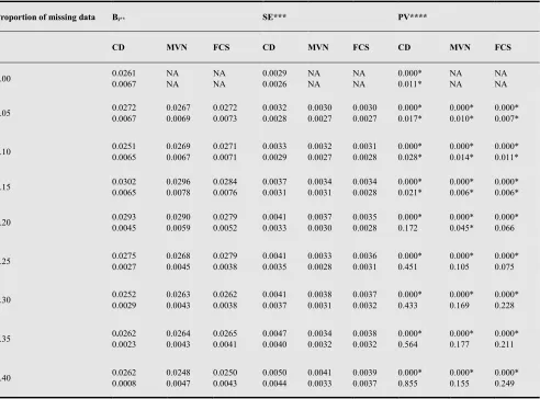
Table 1. Parameter estimates of a set of logistic regression models for predicting the contraceptive methods use status by women of reproductive age in
Democratic Republic of Congo (DRC), using age (1st covariate) and education (2nd covariate) in years as explanatory variables.
Proportion of missing data Bi** SE*** PV****
CD MVN FCS CD MVN FCS CD MVN FCS
0.00 0.0261 0.0067 NA NA NA NA 0.0029 0.0026 NA NA NA NA 0.000* 0.011* NA NA NA NA
0.05 0.0272 0.0067 0.0267 0.0069 0.0272 0.0073 0.0032 0.0028 0.0030 0.0027 0.0030 0.0027 0.000* 0.017* 0.000* 0.010* 0.000* 0.007*
0.10 0.0251 0.0065 0.0269 0.0067 0.0271 0.0071 0.0033 0.0029 0.0032 0.0027 0.0031 0.0028 0.000* 0.028* 0.000* 0.014* 0.000* 0.011*
0.15 0.0302 0.0065 0.0296 0.0078 0.0284 0.0076 0.0037 0.0031 0.0034 0.0031 0.0034 0.0028 0.000* 0.021* 0.000* 0.006* 0.000* 0.006*
0.20 0.0293 0.0045 0.0290 0.0059 0.0279 0.0052 0.0041 0.0033 0.0037 0.0030 0.0035 0.0028 0.000* 0.172 0.000* 0.045* 0.000* 0.066
0.25 0.0275 0.0027 0.0268 0.0045 0.0279 0.0038 0.0041 0.0035 0.0033 0.0028 0.0036 0.0031 0.000* 0.451 0.000* 0.105 0.000* 0.075
0.30 0.0252 0.0029 0.0263 0.0043 0.0262 0.0038 0.0041 0.0037 0.0038 0.0031 0.0037 0.0032 0.000* 0.433 0.000* 0.169 0.000* 0.228
0.35 0.0262 0.0023 0.0264 0.0043 0.0265 0.0041 0.0047 0.0040 0.0034 0.0032 0.0038 0.0032 0.000* 0.564 0.000* 0.177 0.000* 0.211
0.40 0.0262 0.0008 0.0248 0.0047 0.0250 0.0043 0.0050 0.0044 0.0041 0.0033 0.0039 0.0037 0.000* 0.855 0.000* 0.155 0.000* 0.249
*: Significant at 5% level, **: Slopes, ***: Standard errors, ****: P-values.
Figure 1. Estimates of slopes for age when the case deletion (CD), multivariate normal imputation (MVN) and fully conditional specification (FCS) methods
Figure 2. Estimates of slopes for education when the case deletion (CD), multivariate normal imputation (MVN) and fully conditional specification (FCS) methods are used at different rates of missingness.
Figure 3. Estimates of standard errors for age when the case deletion (CD), multivariate normal imputation (MVN) and fully conditional specification (FCS)
methods are used at different rates of missingness.
Figure 4. Estimates of standard errors for education when the case deletion (CD), multivariate normal imputation (MVN) and fully conditional specification
(FCS) methods are used at different rates of missingness.
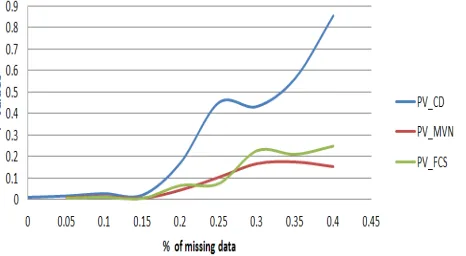
Figure 5. P-values for education when the case deletion (CD), multivariate normal imputation (MVN) and fully conditional specification (FCS) methods are
used at different rates of missingness.
Note that these results did not consider other missingness mechanisms namely the missing at random (MAR) and missing not at random (MNAR) mechanisms. The former states that missingness is related to at least one variable in
mixture of continuous and categorical variables, a study that looks at the performance of these approaches on categorical independent variables that do not assume normality is also needed.
5. Conclusion and Limitations
The MCMC is an iterative procedure used to estimate parameters of interest under difficult conditions such as missing data or when underlying distributions do not fit the assumptions of the maximum likelihood. Its role is to find a probability distribution that can be used to estimate para-meters of interest. This paper discussed the mathematics involved in the data augmentation method based on the multivariate normal model (MVN) that uses the MCMC process. A real dataset (the 2007 DRC DHS) was used to compare inferences made using this method (MVN), the case deletion (CD) missing data technique that discards subjects with missing values from the analysis and the fully conditional specification (FCS) multiple imputation method that uses a sequence of regression models to fill in missing values. The performance of these methods under the as-sumption that data are missing completely at random (MCAR) was highlighted. The results indicated that the higher the proportion of missing data, the more the rela-tionship between variables is distorted when missing data techniques (CD, MVN and FCS) are used. As expected, it was also shown that model-based imputation methods (MVN and FCS) yield less biased estimates than the CD method. Furthermore, the findings indicated that the MVN and the FCS produce similar parameter estimates (van Buuren, 2007) but the MVN is better in terms of preserving an existing relationship between variables at higher rates of missing values. Finally, it was highlighted that at some stage (when the proportion of missing data becomes high, neither the imputation methods nor the case deletion can help to maintain the existing relationship between variables when the analysis is done on the data set with no missing values.
References
[1] Demirtas, H., Freels, S.A. and Yucel, R.M. (2008). Plausi-bility of multivariate normality assumption when multiply imputing non-Gaussian continuous outcomes: a simulation assessment. Journal of Statistical Computation and Simula-tion, 78(1): 69-84.
[2] Enders, C. K. (2010). “Applied Missing Data Analysis”, 1st ed. Guildford Press, New York.
[3] Enders, C.K. (2006). A primer on the use of modern missing data methods in psychosomatic medicine research,
Psycho-somatic Medicine, 68(3): 427-437.
[4] Galati, J. C. and Carlin, J. B. (2008). INORM: Stata Module to Perform Multiple Imputation Using Schafer’s Method [software]. Chestnut Hill, MA: Department of Economics, Boston College, USA.
[5] Gelman, A., Carlin, J.B., Stern, H.S. and Rubin, D.B. (2004). “Bayesian data analysis”, second edition. Boca Raton, Chapman & Hall.
[6] Graham, J.W. (2009). Missing Data Analysis: Making It Work in the Real World, Annual review of psychology, 60: 549–576.
[7] Horton, N.J. and Lipsitz, S.R. (2001). Multiple Imputation in Practice: Comparison of Software Packages for Regression Models With Missing Variables, American Statistical Asso-ciation, 55: 244-254.
[8] Jackman, S. (2000). Estimation and Inference via Bayesian Simulation: An Introduction to Markov Chain Monte Carlo, American Journal of Political Science, 44: 375-404.
[9] Janssen, K.J.M. (2010). Missing covariate data in medical research: To impute is better than to ignore. Journal of clin-ical epidemiology, 63: 721-727.
[10] Lee, K.J. and Carlin, J.B. (2010). Multiple Imputation for Missing Data: Fully Conditional Specification Versus Mul-tivariate Normal Imputation. American Journal of Epidemi-ology, 171(5).
[11] Leeuw, E.D. and Huisman, J. Hox, M. (2003). Prevention and treatment of item nonresponse, Journal of Official Sta-tistics, 19: 153-176.
[12] Little, R. and Rubin, D. (2002). “Statistical Analysis with Missing Data”. John Wiley and Sons Inc, New York.
[13] McKnight, P.E. and McKnight, K.M., Sidani, S. and Fi-gueredo, A.J. (2007). “Missing Data: A Gentle Introduction”. Guilford Press, New York.
[14] Schafer, J.L. (1997). “Analysis of Incomplete Multivariate Data”. Chapman and Hall, London.
[15] Schafer, J.L. and Graham, J.W. (2002). Missing Data: Our View of the State of the Art. Psychological methods, 7(2): 147-177.
[16] Tsikriktsis, N. (2005). A review of techniques for treating missing data in OM survey research. Journal of Operations Management, 24: 53-62.
[17] [van Buuren, S. (2007). Multiple of discrete and continuous data by fully conditional specification. Statistical Methods in Medical Research, 16(3): 219-242.
[18] van Buuren, S. and Knook, D.L. (1999). Multiple Imputation of Missing Blood Pressure Covariates in Survival Analysis. Statistics in Medicine, 18: 681-694.