Application and evaluation of Stanghellini model in the determination of crop evapotranspiration in a naturally ventilated greenhouse

Application and evaluation of Stanghellini model in the determination of

crop evapotranspiration in a naturally ventilated greenhouse

Samuel Joe Acquah

,

Haofang Yan

,

Chuan Zhang

,

Guoqing Wang

,

Baoshan Zhao

,

Haimei Wu

,

Hengnian Zhang

(1. Research Centre of Fluid Machinery Engineering and Technology, Jiangsu University, Zhenjiang 212013, China; 2. Department of Crop & Soil Sciences, Kwame Nkrumah University of Science & Technology, UPO, PMB, Kumasi, Ghana;

3. Institute of Agricultural Engineering, Jiangsu University, Zhenjiang 212013, China; 4. Nanjing Hydraulic Research Institute, Nanjing 210029, China)

Abstract: Stanghellini model is one of the few models primarily developed to predict the evapotranspiration of crops (ETc) in

naturally ventilated greenhouses. However, there are insufficient data on the model regarding its use, particularly in China where solar greenhouses without heating systems are fast spreading for vegetable growth and production. The application of Stanghellini model and the evaluation of its performance using meteorological and tomato plant data generated inside an unheated and naturally ventilated multi-span Venlo-type greenhouse is exploited in this study. Model capability was evaluated by utilizing data from sap flow measurements, meteorological and crop data. Measured meteorological data included solar radiation (Rs),

air temperature (Ta), relative humidity (RH) and net radiation (Rn). Average leaf area index (LAI) values measured during the

experimental period were 1.00, 3.30, 4.05 and 2.93; while determined crop coefficients (Kc) changed from 0.40, 0.62, 1.12 to 0.83

for the initial stage, development stage, mid-season stage and late-season stage, respectively. Results from the study indicated that the average hourly ETc values of tomato plants using sap flow measurements were 0.165 mm/h, 0.148 mm/h, 0.192 mm/h

and 0.154 mm/h for the initial stage, development stage, mid-season stage and late-season stage, respectively. Meanwhile, the

ETc values obtained from calculation using Stanghellini model were 0.158 mm/h, 0.152 mm/h, 0.202 mm/h and 0.162 mm/h for

the initial stage, development stage, mid-season stage and late-season stage, respectively. These ETc values calculated by the

Stanghellini model were close to the measured values within the same period. The coefficients of correlation (R2) based on hourly ETc for the calibration data was 0.94 and that of the validation dataset was 0.90. Scatter plots of the estimated and

measured hourly ETc revealed that the R2 and the slope of the regression line for May, June and July were 0.94, 0.90, 0.96 and

1.15, 0.97, 1.10 respectively. These data were well represented around the 1:1 regression line. A model sensitivity analysis carried out illustrates how the changes in Rs and Ta affect greenhouse ETc. Stanghellini model was therefore proven to be

suitable for ETc estimation with acceptable accuracy in unheated and naturally ventilated greenhouses in the Northeast region of

China.

Keywords: calibration, verification, crop evapotranspiration, naturally ventilated greenhouse, sap flow

DOI: 10.25165/j.ijabe.20181106.3972

Citation: Acquah S J, Yan H F, Zhang C, Wang G Q, Zhao B S, Wu H M, et al. Application and evaluation of Stanghellini model in the determination of crop evapotranspiration in a naturally ventilated greenhouse. Int J Agric & Biol Eng, 2018; 11(6): 95–103.

1 Introduction

Greenhouse crops require adequate irrigation at the right time in order to minimize water stress, and maximize yield and quality

Received date: 2017-11-13 Accepted date: 2018-09-29

Biographies: Samuel Joe Acquah, PhD candidate, research interests: water saving irrigation theory and technology, agricultural water management, agricultural soil, plant and water relations, agricultural science education, Email: 5103160325@stmail.ujs.edu.cn; Chuan Zhang, PhD, Associate Professor, research interests: water saving irrigation theory and technology, agricultural water management, Email: chuan_z@yahoo.com; Guoqing Wang, PhD, Professor, research interests: hydrology and water resources, hydrological modelling, Email: gqwang@nhri.cn; Baoshan Zhao, Graduate student, research interests: water saving irrigation theory and technology, agricultural water management, Email: zhao_baoshan@outlook.com; Haimei Wu, Graduate student, research interests: water saving irrigation theory and technology, agricultural water management, Email: 15051883708@163.com; Hengnian Zhang, Graduate student, research interests: water saving irrigation theory and technology, agricultural water management, Email: zhn349811591@ 163.com. *Corresponding author: Haofang Yan, PhD, Associate Professor, research interests: water saving irrigation theory and technology, agricultural water management. Research Centre of Fluid Machinery Engineering and Technology, Jiangsu University, 301 Xuefu road, Zhenjiang 212013, China. Tel: +86 18252933901, Email: yanhaofang@yahoo.com.

of production. Proper irrigation scheduling and water supply are very important to improve crop yield. Scheduling water application is critical since inaccurate irrigation, especially excessive irrigation may cause waterlogging, root damage and water losses below the root zone[1]_{, and limited irrigation leads to}

weaker plants and poor crop yield[2,3]. Scarcity of water resources requires greenhouse growers to put more emphasis on improving their irrigation strategies so as to provide crops with exact water requirements, effectively reduces water consumption and ensure production. This calls for a better knowledge and understanding of the evapotranspiration process, adapting the water inputs to meet the plant needs. Prediction of ETc depends solely on

meteorological and plant data generated in greenhouse, and accurate estimation of ETc is required to support efficient irrigation

design, planning and scheduling in the greenhouse as well as other models which simulate or attempt to simulate the water-soil budget and improving water use efficiency, in arid and semi-arid regions that rely on irrigation for agricultural production[4]. Applying ETc

models to quantify crop water use in the greenhouse has been a reliable and effective tool in irrigation scheduling[5]_{; greenhouse}

greenhouse ETc must provide timely information for the

implementation of greenhouse water management.

Generally, the most accurate measurement of ETc is

gravimetric method under field conditions, weighing lysimeters-an isolated soil tank mounted on a load cell (electronic weighing balance) that directly measures the evaporation of water from the soil and the loss of water from plant leaves (transpiration) is employed for such purposes[11]. Many greenhouse models have been formulated using either the physical model (i.e. a combination method based on energy balance) - e.g. FAO Penman, 1948; FAO Penman-Monteith, 1998, or the empirical model (i.e. a radiation- based or radiation-temperature based) - e.g. Priestly-Taylor, 1972; FAO Radiation, 1975; Hargreaves-Samani, 1985- to evaluate ETc

and its practical applications in the open field and greenhouse irrigations is to boost vegetable production worldwide.

Greenhouse ETc models commonly used in China to evaluate

crop water requirement included pan evaporation methods for cucumber; tomato in an unheated greenhouse; and Penman-Monteith method for tomato[12-15]_{. In the open fields,}

Penman-Monteith method for ETc in maize and buckwheat fields;

FAO Penman and Priestley-Taylor models for vegetation have been reported[16-20]. All these models differ in the availability of data needed for calculation and their accuracy. Additionally, the coefficients of these greenhouse simplified models depend on wind speed, temperature and stage of crop development. However, in the naturally ventilated greenhouse, wind speed is virtually zero and can lead to large differences in errors in predicted ETc. Thus,

the validity of these models can be compromised and therefore, needed to be checked. However, to date, available data on Stanghellini[21] method for naturally ventilated and unheated greenhouse ETc is scanty. Stanghellini revised the first

evapotranspiration model developed by Penman[22] _{with the}

inclusion of the leaf area index (LAI) term mainly for greenhouse microclimatic conditions. Stanghellini proposed a more elaborate model where the stomatal resistance depends on solar radiation, leaf vapour pressure deficit, leaf temperature and CO2

concentration. The model is a combination equation, which includes the internal and external resistances of the canopy consisting of multi-layers meant for surface evaporation. Available literature on ETc models in greenhouses records that the

best option for the ETc estimation in a naturally ventilated, medium

and high technology greenhouses with no heating systems is the Stanghellini model. This is because the influence of both solar radiation and vapour pressure deficit on the stomatal conductance was taken into account in the formulation of the model[23-25]_.

Several greenhouse studies including comparison of ETc models

using green pepper[26]; acer rubrum tree[27]; and tomato[28,29] have shown higher accuracies with the Stanghellini approach predicting

ETc of greenhouse crops.

However, in all these studies, the influence of wind speed was important in the high performance levels of the model. This study specifically focuses on the application of Stanghellini model to determine ETc under naturally ventilated greenhouse conditions

where wind speed is near or close to 0 in the northeast subtropical region of China; and also evaluate the model’s performance using meteorological and crop data.

2 Materials and methods

2.1 Experimental site

The experiment was conducted in an unheated and naturally ventilated multi-span Venlo-type greenhouse at Jiangsu University

(31°56′N, 119°10′E) located in Zhenjiang City, Jiangsu Province, China, from March 2016 to July 2016. The experimental site is in a humid sub-tropical monsoon climatic zone with an average annual air temperature of 15.5o_{C and a mean annual precipitation}

(rainfall) of 1058.8 mm, relative humidity is 76 % at 26 m above sea level. The rectangular greenhouse structure has an area of 32 m long × 20 m wide in horizontal dimensions, 3.8 m high with the longer side in an east-west orientation, which is the prevailing wind direction. Greenhouse operates on natural ventilation for the exchange of hot exhaust air from the inside of the greenhouse to the outside. Heating system available in the greenhouse is non-functional. The planting medium used in the greenhouse was a soil-biochar mixture with mean bulk density of 1.266 g/cm3, field capacity of 0.408 cm3/cm3 and permanent wilting-point water content of 0.16 cm3/cm3 in the depth of 0-60 cm.

2.2 Design, materials and greenhouse meteorological data measurements

Tomato (Lycopersicon esculentum L. cv. Jinzuan-3), which is one of the main cultivars of tomato in the province, was used for this study and planted in 9 plots with 54 plants planted in two rows between March to July 2016 (as shown in Table 1). Each soil box was 0.65 m long × 0.45 cm wide. Seedlings were sowed 30 days before transplanting. Prior to transplanting, the soil-biochar planting medium was prepared to ensure proper uniform mixture of soil and biochar in the soil boxes. Transplanting was done with a planting density of 2 plants per soil box evenly spaced at 0.40 m apart. For a better establishment and to ensure seeding growth, the transplanted seedlings were immediately irrigated with the same volume of water (25 mm). Thereafter, the plants were watered by drip irrigation and the spatial interval of the emitters in each drip tape was 0.35 m. The designed discharge rate of each drip tape was 100 mL/min. Drip surface irrigation application was initiated 3 days after transplanting (DAT) together with 200 ppm fertilizer solution applied directly to the tomato plants. Specific concentrations of NPK were 25 % N, 5 % P2O5 and 5 %

K2O. All treatments were given the same agronomic management

practices such as pruning branch stem, fertilization, pest control and trellised support. Following the FAO-56 approach, the growth season of the tomato crop is divided into four stages: the initial stage, the crop development stage, the mid-season stage and the late season stage[30]. The divided growth stages for the tomato crop, main features and the duration of each stage are presented in Table 1.

Meteorological data inside the greenhouse were measured using a standard automatic weather station located inside the greenhouse. Solar radiation (Rs), air temperature (Ta), relative

humidity (RH) and net radiation (Rn) were the meteorological

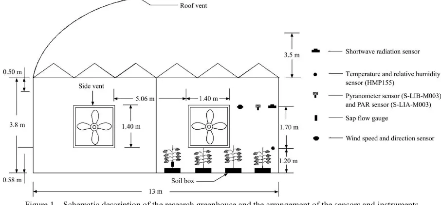
parameters collected over the whole growing season inside the greenhouse. The elements of air temperature and relative humidity were measured both at 1.20 m and at 2.90 m heights from the ground level, respectively (as shown in Figure 1). Humidity and temperature sensors HMP155 (Vaisala HUMICAP, Vaisala Oyj, Finland) were used for the measurements. A silicon pyranometer sensor S-LIB-MOO3 (OnsetCom, USA) placed above the tomato crop canopy was used to measure the incoming shortwave solar radiation and net radiation measured by a net radiometer, NR Lite 2 (Kipp & Zonen, Delft, The Netherlands) with sensitivity of 15.3 μV/(W m-2). Sensor specifications for Ta,

RH, Rn, and Rsare –20°C-60°C, 0-100%, 0-2000 W/m 2

and 0- 2000 W/m2_{, with the precision values of ±0.1°C, ±2%, ±2% and}

10 s, averaged every 10 min and recorded by two computer- controlled data loggers CR1000 (Campbell Scientific, USA) and

HOBO U30 (Station Remote Monitoring Systems, OnsetCom, USA).

Figure 1 Schematic description of the research greenhouse and the arrangement of the sensors and instruments

2.3 Tomato crop transpiration measurements

Tomato crop transpiration was determined using a sap flow system (Flow32-1K Sap Flow System, Dynamax Inc., Houston, TX, USA). In each plot, the SGA-WS gauges of the sap flow (Dynamax Inc., Houston, TX, USA) were installed at representative plants of the tomato crops. Twelve healthy plants were selected and their stem diameters were measured prior to installation of gauges. Stem diameters measured ranged from 5.07 mm to 12.47 mm. The SGA2-WS, SGA5-WS, SGA7-WS and SGA9-WS gauges were used to measure the sap flow, gauges were fixed on the stems 20 cm above the ground surface to avoid the effect of surface heat flux[23,24]. Sap flow from 23 May to 23 July, 2016 were measured, and the sap flow data was collected after every 10 min by a data logger CR1000 (Campbell Scientific Inc., USA).

Table 1 Growth stages for tomato during the entire experimental period

Growth stage Main feature Date Duration

/d Initial Seedling and vegetative stage 03/03/16-18/03/16 15 Development Flowering and fruit formation 19/03/16-20/04/16 42 Mid-season Fruit development and maturation 21/04/16-23/06/16 63 Late season Breaker to full ripe and final

harvest stage 24/06/16-23/07/16 29 The sap flow of each individual plant was then converted to plant transpiration using the following formula by Gong et al.[25]:

1

1 /

[ ]

1000

n _{i i}

i

f LA

T LAI

n







where, T is the plant transpiration after normalizing the sap flow data by the leaf area, mm/h; fi is the stem flow, g/h; LAi, the leaf

area, m2; n is the number of plants measured; and LAI, leaf area index, m2/m2.

2.4 Leaf area index, plant height and crop coefficients

Manual non-destructive method of LAI measurements were done at an interval of 5-14 days. Eighteen healthy plants were sampled from the 9 plots. The leaf length (L) and the highest leaf width (WL) were measured with a measuring tape, and the

conversion coefficient of 0.657 for the leaf area was derived by

fitting the measured results to the one drawn using CAD software[31]. LAI was determined as follows:

1

[ ] 0.657

n _L

i

R P

L W LAI

I I



   

  _ 

 



where, IP is the average distance between two closest or

neighbouring plants (inter-plant distance = 0.40 m), and IR is the

average row space (inter-row distance = 0.45 m). Leaf area index was defined as the ratio between total leaf area and the ground area of the whole canopy, it was extrapolated from the above formula and used as an input in the Stanghellini model calibration and validation. Plant height was measured with the 18 healthy tomato plants at same time of leaf area measurements.

The crop coefficient (Kc) values for the tomato crop for any

period of the growing season were determined on the assumption that Kc is constant and equal to the Kc value of the growth stage

during the initial and mid-season stages. In addition, during the crop development and late season stages, Kc varies linearly

between the Kc at the end of the previous stage (Kc prev) and the Kc

at the beginning of the next stage (Kc next), that is, Kc end, in the case

of the late season stage. Thus, Kc values were determined as

follows:

( )

( )

prev

c i c prev c next c prev

stage

i L

K K K K

L

   

   

 

  (3)

where, i is day number within the growing season (L…length of growing season); Kc i is the crop coefficient on day i; Lstage is length

of the growing stage under consideration (days); ∑(Lprev) is sum of

the lengths of all previous stages (days)[30]_{. Equation (3) can be}

applied to all four growth stages outlined in Table 1.

2.5 Stanghellini model based on hourly time scale

The hourly Stanghellini model of the crop evapotranspiration,

ETcis basically a revised Penman-Monteith model representing

greenhouse microclimatic conditions of typically low wind speed (u˂1.0 m/s; for naturally ventilated greenhouses, u≈0 m/s) and low

solar radiation. Hourly climatic data measured inside a Venlo-type greenhouse with natural ventilation was used to calculate the hourly ETc. The Stanghellini model includes

absorption in a multi-layer canopy[26,32]. This model was developed specifically for the conditions of a greenhouse utilize

LAI to account for energy exchange from multiple layers of leaves on the greenhouse tomato crop. According to Villarreal-Guerrero et al.[29], the LAI in the Stanghellini model has significant effect on the accuracy of the model. The Stanghellini equation for hourly

ETc (mm/h) is defined by Donatelli et al.[33] and described as

follows:

Δ( )

1 2

Δ (1 )

p n t R c c C a

VPD ρ C

R G K

r ET K LAI

r λ _γ r                 _{ }         (4) 0

252 ( )

0.07 ns p a

n

R

R ρC T T

R

r

 

 (5)

0.07

ns s

R  R (6)

3

4 ( 273.15)

p R a ρc r σ T 

 (7) where, ETc is crop evapotranspiration under standard

conditions,(mm/h; Rn is net radiation at the crop surface, (MJ·m2)/h;

Rns is net short wave radiation, (MJ·m2)/h; Rs is ground level solar

radiation, (MJ·m2_{)/h; K}

tis time unit conversion factor equal to

3600 s/h; Tais mean hourly air temperature at 2 m height, °C; T0 is

leaf temperature, °C; VPD is hourly vapour pressure deficit, kPa;

LAI is leaf area index, m2/m2; G is soil heat flux density, (MJ·m2)/h; Δ is slope of the saturation vapour pressure curve, kPa/°C; γ is psychrometric constant; ρ is mean atmospheric density, kg/m3; λ is latent heat due to water vaporization, kJ/kg; cp is specific heat

capacity of air at constant pressure, MJ/(kg·°C); rR is radiative

resistance, s/m; ra is aerodynamic resistance, s/m; rc is canopy

(stomatal) resistance, s/m; σ is Stefan-Boltzman constant, MJ/(m2 K4·h), and Kc is the crop coefficient mainly affected by

crop type, crop height, albedo (reflectance) of the crop-soil surface, aerodynamic properties, leaf properties and crop stages[30].

A summary of Stanghellini model input variables used in the calculation[33] is shown in Table 2.

2.6 Estimation of aerodynamic resistance

In greenhouse, the heat and mass transfer between vegetation and interior air are largely dependent on the aerodynamic resistance (ra). The determination of the transfer of heat and water vapour

from the evaporating surface into the air above the canopy is referred to as ra. The ra is mainly related to a mean interior air

speed, assumed constant in most energy balance models. However, this is only true when the greenhouse is closed or when natural ventilation is maintained at a small and constant value as reported by Wang et al.[34] The ra, mainly depends on the

aerodynamic regime that prevails in the greenhouse. Considering that the buoyancy force can be ignored with respect to the wind force, ra can be directly expressed with respect to the average

interior air speed expressed by Boulard and Wang[35] as follows: 0.2 0.8 220 a i d r V

 (8)

where, d is the characteristic length of the leaf (m); Vi, the mean

interior air speed, m/s, can be considered to be proportional to the ventilation flux Փv divided by Ac, m2, the vertical cross-section area

perpendicular to the average direction of the inside air flux, in this case the greenhouse axis, expressed as[36]:

i c

v V

A

 (9)

Table 2 Variables used in the Stanghellini model

Variable Unit Symbol Equation

Latent heat of vaporization MJ·kg-1 λ λ=2.501–0.002361Ta

Soil heat flux MJ·m2·h-1 G G = measured values

Net radiation MJ·m2·h-1 Rn 252 ( 0)

0.07

n

ns p a

R

R

R ρ C T T r



    

Net short wave radiation MJ·m2·h-1 Rns Rns0.77Rs

Specific heat of the air MJ·kg-1·°C-1 Cp Cp0.001013

Mean atmospheric

density kg·m

-3 _ρ 100000

(a 273.16)

ρ R T

 

Specific gas constant J·kg-1_·K-1 _R

287

R

Actual vapour pressure kPa ea

100

a s

RH e e

Saturation vapour

pressure kPa es

( ) 6.894757 f R s

e  e

Function of air

temperature - f(R) 5 2

9 3 10440

( ) 11.29

0.02702 1.289 10 2.478 10 6.546 ln( )

a a a a a f R T T T T T           

Air temperature °C Ta Ta = measured values

Leaf temperature

(Daytime) °C T0 0 a 1.67 s 0.25

VPD T T R

γ

  

Leaf temperature

(Nighttime) °C T0 0 a 0.1

VPD T T γ        

Slope of the saturation

vapour pressure curve kPa·°C

-1 _{Δ Δ 0.04145}0.06088T

e



Vapour pressure deficit kPa VPD VPD es ea

Psychrometric constant kPa·°C-1 γ _γ C ρp

ελ



Water to dry molecular

weight ratio - ε ε0.622

Aerodynamic resistance s·m-1 _r

a Refer to Equations (8)-(10)

Internal resistance s·m-1 ri Refer to Equation (11)

Radiative resistance s·m-1 rR 3

4 ( 273.15)

p R a ρC r σ T  

Boulard and Baille[36] explained that the relationship accounting for the combination of thermal and wind effects used to calculate the ventilation flux (Փv in m3/s) is given as:

2 3/ 2 2 3/ 2

0 _[( Δ _{) ( ) ]}

3 Δ d e

w e w e

e

L C T g T

v h C U C U

g T T

   (10)

where, Cd and Cw are empirical discharge and wind effect

coefficients, identified for this greenhouse as 0.644 and 0.09[36]_,

respectively; g is acceleration due to gravity constant, m/s2; h is the vertical height of the vent opening, m; L0 is the length of the

continuous vents, m; Te and ∆T are the exterior air temperature and

the interior-exterior air temperature difference (K) and Ue is the

external wind speed, m/s.

2.7 Estimation of internal resistance

The internal resistance, ri refers to the average resistance of an

crop ages and begins to ripen. Avissar et al.[3] have reported that the internal resistance can be considered to be dependent on the inside level of global radiation and inside air temperature and humidity based on exponential laws. For greenhouse tomato crops, the effects of radiation on internal resistance are the most crucial and obey the relationship given by Boulard and Wang[35] _as

follows:

1

200(1 )

exp(0.05( 50))

i

g

r

τR

 

 (11) where, τ is the transmittance of the greenhouse cover; and Rg is the

outside global solar radiation, W/m2.

2.8 Model calibration and verification

The entire measurement period was divided into sky-clear and cloudy days. Calibration (8-31 May 24 consecutive days); verification (2-24 June 24 consecutive days); and model sensitivity analysis were carried out only in the sky-clear days to show the model response to variations in the major meteorological variables like Ta, Rsand VPD. Data obtained during the calibration period

were used to derive a set of regressions related to the calculated variables: measured Rs,,Ta and ETc were regressed against their

corresponding calculated values. During the verification period calculated values of Rs,,Ta and ETc were verified against their

corresponding measured ones by linear regression.

2.9 Sensitivity analysis

A model sensitivity analysis was carried out to further validate and evaluate the model response to variations in the major meteorological variables (in this case solar radiation, Rs, VPD and

air temperature, Ta). In order to simulate the performance of the

model under different monthly climatic conditions, the sensitivity of the model to simultaneous changes in Rs, VPD and Ta was

examined.

2.10 Statistical analysis

The measured and calculated ETc were compared by using

simple error analysis and linear regression. For each month, the following parameters were calculated: mean absolute error (MAE), root mean squared error (RMSE), and the percent deviations of average measured and calculated ETc (% Deviations).

Additionally, maximum, minimum, mean and standard deviations for each month were also calculated. For validation of the Stanghellini model, the statistical error between measured and calculated ETc was calculated and two-tail t-test statistical analysis

method was used with the data from July, 2016.

3 Results and discussion

3.1 Variations of plant height and LAI

The active LAI describes the index of the leaf area or healthy leaves actively contributing to the surface heat and vapour transfer. The variations of crop height and LAI of tomato during the experiment is shown in Figure 2. The tomato plant reached a maximum height of 1.84 m at approximately 90-110 d after transplanting (DAT). The maximum plant height was higher than the value (=1.56 m) reported by Harmanto et al.[38] using Troy 489 tomato variety. The measured LAI exceeded 1.0 around 50 DAT

and reached a maximum value of 4.05 in the experimental duration. The LAI was assumed not to change significantly within a week and a constant weekly value was used for the model calibration and validation.

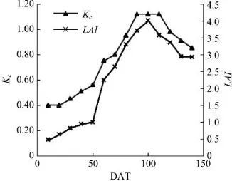
3.2 Daily crop coefficients

Crop coefficients (Kc) determined using Equation (3) as

suggested by Allen et al.[30], ranged from 0.40 to 1.12. At the start

of the experimental study, Kc (initial) was 0.40. During canopy

development (crop development stage), Kc (dev.) increased rapidly

reaching 0.95 at mid-season stage of crop development. Kc (mid)

remained relatively constant, varying from 0.95 to the peak of 1.12 (as shown in Figure 3). The average mid-season Kc was similar to

values reported by Phene et al.[39] for tomato plants grown under similar conditions. The daily crop coefficient data showed well-defined late-season growth stages (Kc (end)) with values

decreasing from 0.92 to 0.83. Initially, the Kc was increased

almost linearly from 0.40 to reach a maximum value of 1.12 (Kc (mid)) when LAI was slightly above 4.0. Finally, Kc decreased

slightly down to 0.8 at the end of the growth season which was associated with a decline in LAI as illustrated in Figure 3.

Figure 2 Evolution of tomato plant height and LAI during the experimental period

Figure 3 Curves of crop coefficient (Kc) and LAI of tomato plant

during the experimental period (March to July, 2016)

3.3 Evaluation of aerodynamic and internal resistances

Stanghellini[21] reported that relatively small variations in wind movement within the greenhouse result in a fairly constant aerodynamic resistance. However, previous reports have shown that authors often choose a constant value for the aerodynamic resistance since there is not much loss of accuracy in using a constant value[29,40]_{. The predicted ET}

c was found to be

practically ‘not sensitive’ to the leaf aerodynamic resistance. This finding is in agreement with results reported for the evaluation of transpiration with a constant aerodynamic resistance[10,27]. In the present study, Equations (8)-(10) were employed for the determination of the aerodynamic resistance in an attempt to improve the accuracy of the ETc predictions. Results indicated

reported for tomato in greenhouse conditions[21,29,41].

Figure 4 Hourly behaviour of aerodynamic and internal resistances

The internal resistance was calculated using Equation (11). Solar radiation has strong and effective impact on internal resistance and was found to be high during the early hours of the day and in the night hours. The main reason for this pattern can be attributed to the stomatal closures during those hours. During the night, stomata remain closed resulting in higher resistances to the water vapour transfer. In the presence of solar radiation, the stomata open for photosynthesis, thus drastically reduce the internal resistance[29,41-43]. The internal resistance values determined in this study were high due to the LAI term prevalent in Equation (4) with coefficient of 2, thus, affecting the output of the internal resistance. The consistently higher values of the internal resistance obtained were in agreement with values reported in literature for a greenhouse cooling strategy with natural ventilation[29].

3.4 Evaluation of greenhouse meteorological variables

Table 3 is the summary of the maximum, minimum, mean and standard deviations of hourly averages for the three consecutive months May, June, and July of all meteorological parameters

measured in the greenhouse (RH, Ta, Rn and Rs) from 8 May to 23

July, 2016. The average minimum Rn remained constant at

0.60 W/m2 for the 3 months whereas the average maximum recorded values were 403.9 W/m2, 497.9 W/m2 and 589.4 W/m2 for May, June and July, respectively. Average minimum values for Rswere

19.6, 11.9 and 12.4 with the maximum of 726.9 W/m2, 598.0 W/m2 and 621.5 W/m for May, June and July, respectively. The average minimum Ta recorded values were 14.1, 20.2 and 22.9, and the

maximum were 43.4°C, 42.8°C and 52.3°C for May, June and July. Average minimum RH values were 25.6%, 43.0% and 37.3% for May, June and July, respectively, whilst the maximum was 100 % for all the 3 months. The differences were mainly due to varied solar radiation during the experimental period in the greenhouse.

Table 4 present the estimated and measured hourly ETc using

the sap flow measurements from 23 May to 23 July 2016. The calculated ETc was derived from Stanghellini model calculations

using meteorological and crop data. The measured ETc was

obtained from sap flow measurements when the soil surface was almost covered by canopy and after normalizing the sap flow data by the leaf area. The hourly ETc calculated for May, June and

July increased linearly as Rs(ETc = 0.35Rs – 0.67, R 2

= 0.90), Ta

(ETc = 0.25Ta – 2.67, R2 = 0.76), Rn (ETc = 0.41Rn– 2.25, R2 =

0.79), and RH (ETc = 1.35RH + 0.25, R2 = 0.63). The hourly ETc

was significantly influenced by Rs, Rn, Ta and RH (p˂0.001), and

the correlation between hourly ETc and Rs was higher compared

with Rn, and Ta, but inversely with RH. The Rs appeared to be the

main meteorological variable determining the greenhouse ETc.

Similar assessments were made by Qiu et al.[23], Fernández et al.[44] and Jiao et al.[45] with the conclusion that the relationship between

Rs and Rn varies with greenhouse Ta. The measured and calculated

diurnal variations of Rn for May, June and July are shown in

Figures 5a-5c.

Table 3 Greenhouse maximum, minimum, mean and standard deviations of RH, Rn, Ta and Rs of hourly averages for May,

June and July 2016

Parameter

May June July

Min Max Mean SD Min Max Mean SD Min Max Mean SD

Rn /W·m-2 0.60 403.97 37.82 70.84 0.60 497.92 37.25 67.30 0.60 589.38 57.60 105.10

Rs/W·m-2 19.56 726.90 65.66 130.87 19.56 726.90 65.66 130.87 12.45 621.50 62.36 115.19

Ta /°C 14.10 43.36 22.66 7.02 20.16 42.81 28.77 5.55 22.93 52.33 31.51 6.88

RH /% 25.63 100.00 73.46 21.45 43.03 100.00 83.94 15.68 37.28 100.00 82.16 18.63 Note: Min, Max and SD are minimum, maximum, and the standard deviations, respectively, of hourly averages of all meteorological data recorded for May, June and July 2016 in the greenhouse during the experiment.

Table 4 Error analysis statistics of the comparison between measured and calculated ETc during the experiment in May,

June and July 2016

May June July

Measured ETc /mm·h-1 0.192 0.148 0.154

Calculated ETc /mm·h-1 0.223 0.164 0.171

Slope 1.15 0.97 1.10

Coefficient of correlation/R2 0.94 0.90 0.96

RMSE /mm·h-1 _{0.037 0.019 0.020}

MAE /mm·h-1 0.032 0.018 0.018

Deviations /% 14.16 10.08 9.91

a. May

b. June

c. July

Figure 5 Diurnal courses of net radiation (Rn) for May, June and July

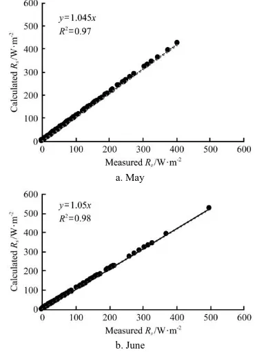
3.5 Calibration and verification of model input data

The results of calibration and verification of the major model parameter Rs are presented in Figures 6a, 6b. Figure 6a represents

the model calibration regression equations using Rs data during the

24 consecutive days in May. Similarly, Figure 6b shows the verification linear regression between the calculated and the measured values using Rs data during the 24 consecutive days in

June. All the calculated variables were well correlated with the corresponding measured variables inside the greenhouse during May and June with the R2≥0.97.

The results of the error analysis statistics of the comparison between hourly measured and calculated ETc data for May and

June, 2016, are shown in Table 4. Figure 7a shows the comparison between measured and calculated ETcfor May. There

was high correlation between measured and calculated ETc. The

regression lines were close to 1:1, which indicates the calculated

ETc were close to the measured values. The coefficient of

determination (R2) was 0.94. Figure 7b represents the comparison between measured and calculated ETcfor June. A high correlation

between measured and calculated ETc resulted in a high coefficient

of determination (R2) of 0.90. Table 4 shows the other statistical parameters, such as mean absolute errors (MAE), root mean squared errors (RMSEs), deviations and regression equations. According to two-tail t-test statistical analysis (significant level α = 0.05), there were no significant differences between measured and

calculated ETc values in all the months under consideration.

a. May

b. June

Figure 6 Comparison of calculated Rs with measured using

a. May

b. June

Figure 7 Comparison of daily ETcbetween Stanghellini model

(calculated ETc) and sap flow measurements (measured ETc) in:

May and June based on only sky-clear days within the months under consideration

3.6 Sensitivity analysis

Sensitivity analysis further evaluated the performance of the model and indicated the change in the ETc due to variations in Ta

and Rs. Figure 8 illustrates the sensitivity test for calculated ETc

obtained by employing Stanghellini model calculations with measured values derived by sap flow measurements in July. The sensitivity coefficient of determination, R2 of 0.96 is in agreement with the calibration and verification R2 of 0.90 and 0.96, respectively. Higher sensitivity of a model suggests that small errors in the measurements of the meteorological parameters may result in larger errors in the ETc prediction[1]. As anticipated from

Equations (4) and (5), ETc increases linearly with Rn and hence Rs

and non-linearly towards Ta. Since sensitivity of the model

increases with increasing ETc and Rs and decreases with Ta, it

implies that the model is more susceptible to changes in the radiation levels in the greenhouse. The model was found to be most sensitive to the level of incoming Rs, followedby Ta

and

Note: ref means Rs = Rs ref, VPD = VPDref and Ta = Taref. The relative change of

ETc (i.e. ETc/ETc ref) is plotted against the relative variations of Rs, VPD and Ta. Figure 8 Result of sensitivity analysis

VPD as shown in Figure 8. Model sensitivity analysis indicated that reduced Rs and Ta were the main meteorological factors

influencing transpiration in the greenhouse.

4 Conclusions

This study calibrated and tested the potential performance of the Stanghellini model for prediction of ETc using meteorological

and crop data generated inside an unheated and naturally ventilated multi-span Venlo-type greenhouse in a sub-tropical climatic environment. Stanghellini model was developed primarily for crops grown under greenhouse microclimatic conditions, particularly where the plant canopy consists of multi-layered surfaces for evaporation. Tomato was used in this study, and results indicated that the hourly ETc measured values were close to

the values predicted by the Stanghellini model during the experimental period. The calibration data had coefficient of correlation (R2_{) to be 0.94 and that of the verification dataset was}

0.90.

Scatter plots revealed that the hourly calculated values from Stanghellini model and measured ETc data were well represented

around the 1:1 regression line. Sensitivity analysis, which evaluated the performance of the model resulted in sensitivity coefficient of determination R2 of 0.96, which was in agreement with the calibration and verification R2 of 0.90 and 0.96, respectively. Model sensitivity analysis showed reduced Rs and

Ta mainly influenced transpiration in the greenhouse. A two-tail

t-test statistical analysis (significant level α = 0.05) revealed that there were no significant differences between measured and calculated ETc. This study revealed that the application of

Stanghellini equation from detailed meteorological data for estimation of ETc in an unheated and naturally ventilated

greenhouse was feasible.

Acknowledgements

We greatly appreciate the careful and precise reviews by the anonymous reviewers and editors. This study has been financially supported by the National Key Research and Development

Program of China (grant number 2016YFA0601501,

2016YFC0400104), the Natural Science Foundation of China (51509107, 51609103); Natural Science Foundation of Jiangsu province (BK20150509), and a project funded by the Priority Academic Program Development of Jiangsu Higher Education Institutions.

[References]

[1] Pirkner M, Dicken U, Tanny J. Penman-Monteith approaches for estimating crop evapotranspiration in screenhouses – A case study with table–grape. International Journal of Biometeorology, 2014; 58(5): 725–737.

[2] Sam-Amoah L K, Darko R O, Owusu-Sekyere J D. Calibration and validation of aqua crop for full and deficit Irrigation of hot pepper. ARPN Journal of Agricultural and Biological Science, 2013; 8(2): 175−178.

[3] Wang S, Fan Z, Gao Y, Li J. Effect of nutrient solution irrigation volume and frequency on winter and spring pepper under soilless cultivating conditions. Journal of Drainage and Irrigation Machinery Engineering, 2018; 36(1): 69–76. (in Chinese)

[4] Yan H F, Zhang C, Oue H, Peng G J, Darko R O. Determination of crop and soil evaporation coefficients for estimating evapotranspiration in a paddy field. Int. J. Agric & Biol Eng., 2017; 10(4): 130–139.

[6] Lorenzo P, Medrano E, Sánchez-Guerrero M C. Greenhouse crop transpiration: an implement to soilless irrigation management. Acta Hort., 1998; 458, 113–119.

[7] Seginer I. The Penman–Monteith evapotranspiration equation as an element in greenhouse ventilation design. Biosyst. Eng., 2002; 82, 423–439.

[8] Li Y, Stanghellini C, Challa H. Effect of electrical Conductivity and transpiration on production of greenhouse tomato (Lycopersicon esculentum L.). Scientia Horticulturae, 2001; 88, 11–29.

[9] Baille A, González-Real M M, Gázquez J C, López J C, Pérez-Parra J J, Rodríguez E. Effects of different cooling strategies on the transpiration rate and conductance of greenhouse sweet pepper crops. Acta Horticulturae, 2006; 719, 463–470.

[10] Kittas C, Katsoulas N, Baille A. Transpiration and canopy resistance of greenhouse soilless roses: measurements and modeling. Acta Horticulturae, 1999; 507, 61–68.

[11] López-Cruz I L, Olivera-López M, Herrera-Ruiz G. Simulation of Greenhouse tomato crop transpiration by two theoretical models. Acta Hort. (ISHS), 2008; 797.

[12] Yin C, Fei L, Liu L, Dai Z, Liu L, Wang A. Effects of water-fertilizer coupling on physiological characteristics of facility planting cowpea. Journal of Drainage and Irrigation Machinery Engineering, 2018; 36(3): 267–276. (in Chinese)

[13] Marek T, Piccinni G, Schneider A, Howell T, Jett M, Dusek D. Weighing lysimeters for the determination of crop water requirements and crop coefficients. Applied Engineering in Agriculture, 2006; 22, 851–856.

[14] Lascano R J. The Soil-plant-atmosphere system and monitoring technology. In: Lascano R J and Sojka R E, Eds., Irrigation of Agricultural Crops, American Society of Agronomy, Crop Science Society of America, and Soil Science Society of America, Madison, 2007; 85–115. [15] Lascano RJ, Duesterhaus JL, Booker JD, Goebel TS, Baker JT. Field

measurement of cotton seedling evapotranspiration. Agricultural Sciences, 2014; 5, 1237–1252.

[16] Yan H, Zhang C, Oue H, Wang G, He B. Study of evapotranspiration and evaporation beneath the canopy in a buckwheat field. Theor. Appl. Climatol., 2015; 122, 721–728.

[17] Yan H, Shi H, Oue H, Zhang C, Xue Z, Cai B, Wang G. Modelling bulk canopy resistance from climatic variables for predicting hourly evapotranspiration of maize and buckwheat. Meteorology Atmos. Phys., 2015b; 127, 305–312.

[18] Liu X, Lin E. Performance of the Priestley-Taylor equation in the semiarid climate of North China. Agricultural Water Management, 2005; 71, 1–17.

[19] Zhang Z, Liu S, Liu S, Huang Z. Estimation of cucumber evapotranspiration in solar greenhouse in Northeast China. Agricultural Sciences in China, 2010; 9(4): 512–518.

[20] Liu H, Duan A, Li F, Sun J, Wang Y, Sun C. Drip irrigation scheduling for tomato grown in solar greenhouse based on pan evaporation in North China Plain. Journal of Integrative Agriculture, 2013; 12 (3): 520–531. [21] Stanghellini C. Transpiration of greenhouse crops: An aid to climate

management. PhD dissertation, Agricultural University of Wageningen, 1987. The Netherlands. 150 pp.

[22] Penman H L. Natural evaporation from open water, bare soil and grass. Proc. Roy. Soc. London A193, 1948; 120–146.

[23] Qiu R J, Kang S Z, Du T S, Tong L, Hao X M, Chen R Q, et al. Effect of convection on the Penman-Monteith model estimates of transpiration of hot pepper grown in solar greenhouse. Scientia Horticulturae, 2013; 160, 163–171.

[24] Qiu R J, Du T S, Kang S Z, Chen R Q, Wu L S. Influence of water and nitrogen stress on stem sap flow of tomato grown in a solar greenhouse. Journal of the American Society for Horticultural Science, 2015; 140(2): 111–119.

[25] Gong X, Liu H, Sun J, Gao Y, Zhang X, Jha S K, et al. A proposed surface resistance model for the Penman-Monteith formula to estimate evapotranspiration in a solar greenhouse. Journal of Arid Land, 2017;

9(4): 530–546.

[26] Jolliet O, Bailey B J. The effect of climate on tomato transpiration in greenhouse: measurements and models comparison. Agric. For. Meteorol., 1992; 58, 43–63.

[27] Prenger J J, Fynn R P, Hansen R C. A comparison of four evapotranspiration models in greenhouse environment. Transactions of the ASAE, 2002; 45, 1779–1788.

[28] López-Cruz I L, Olivera-López M, Herrera-Ruiz G. Simulation of Greenhouse tomato crop transpiration by two theoretical models. Acta Hort (ISHS), 2008; 797.

[29] Villarreal-Guerrero F, Kacira M, Fitz-Rodríguez E, Kubota C, Giacomelli G A, Linker R, et al. Comparison of three evapotranspiration models for a greenhouse cooling strategy with natural ventilation and variable high pressure fogging. Scientia Horticulturae, 2012; 134, 210–221.

[30] Allen R G, Pereira L S, Raes D, Smith M. Crop evapotranspiration: guidelines for computing crop water requirements. In: FAO Irrigation and Drainage Paper No. 56. 1998. FAO, Rome, Italy, 300 pp.

[31] Liu H, Sun J S, Duan AW, Sun L, Liu Z G, Shen X J. Experiment on soil evaporation of radish in sunlight greenhouse. Transactions of the CSAE, 2009; 25(1): 176–180. (in Chinese).

[32] Kirnak H, Short T H. An evapotranspiration model for nursery plants grown in a lysimeter under field conditions. Turkish Journal Agric. For., 2001; 25, 57–63.

[33] Donatelli M, Bellocchi G, Carlini L. Sharing knowledge via software components: Models on reference evapotranspiration. European Journal of Agronomy 24, 186–192.

[34] Wang S, Boulard T, Haxaire R. Air speed profiles in a naturally ventilated greenhouse with a tomato crop. Agricultural and Forest Meteorology, 1999; 96(4): 181–188.

[35] Boulard T, Wang S. Greenhouse crop transpiration simulation from external climate conditions. Agricultural and Forest Meteorology, 2000; 100, 25–34.

[36] Boulard T, Baille A. Modeling of air exchange rate in a greenhouse equipped with continuous roof vents. Journal of Agric. Eng. Res., 1995; 61, 37–48.

[37] Avissar R, Avissar P, Mahrer Y, Bravdo B A. A model to simulate response of plant stomata to environmental conditions. Agricultural and Forest Meteorology, 1985; 34, 21–29.

[38] Harmanto, Salokhe V M, Babel M S, Tantau H J. Water requirement of drip irrigated tomatoes grown in greenhouse in tropical environment. Agricultural Water Management, 2005; 71(3): 225–242.

[39] Phene C J, McCormick R L, Miyamoto J M. Evapotranspiration and crop coefficient of trickle irrigated tomatoes. Proceedings of the Third International Drip/Trickle Irrigation Congress, Nov. 18–21, 1985. Fresno, CA.

[40] Morile B, Migeon C, Bournet P E. Is Penman-Monteith model adapted to predict crop transpiration under greenhouse conditions? Application to a New Guinea Impatiens crop. Scientia Horticulturae, 2013; 152, 80–91. [41] Zhang L, Lemeur R. Effect of aerodynamic resistance on energy balance

and Penman-Monteith estimates of evapotranspiration in greenhouse conditions. Agricultural and Forest Meteorology, 1992; 58(3-4): 209–228.

[42] Yang X, Short T H, Fox R D, Baurle W L. Transpiration, leaf temperature and stomatal resistance of a greenhouse cucumber crop. Agricultural and Forest Meteorology, 1990; 51(3-4): 197–209.

[43] Montero J I, Anton A, Munoz P, Lorenzo P. Transpiration from geranium grown under high temperatures and low humidities in greenhouses. Agricultural and Forest Meteor ology, 2001; 107, 323–332. [44] Fernández M D, Bonachela S, Orgaz F, Thompson R, Lopez J C, Granados M R, et al. Measurement and estimation of plastic greenhouse reference evapotranspiration in a Mediterranean climate. Irrigation Science, 2010; 28, 497–509.