An Augmented Lagrangian Algorithm for Engineering Optimization by Solving Nonlinear Programming Problem

Volume 4 • Issue 4 • October 2018

ISSN 2206-4451

www.ajbssit.net.au

An Augmented Lagrangian Algorithm for Engineering

Optimization by Solving Nonlinear Programming Problem

Mamun-Or-Rashid1 and Syed Anayet Karim2

1_{Faculty of Business Administration, BGC Trust University Bangladesh, Chittagong, Bangladesh,} 2_{Department of} Natural Science, Port City International University, Chittagong, Bangladesh

1. Introduction

In this paper, we discuss about the Augmented Lagrangian Method (ALM) and its algorithm in engineering optimization which has many other interesting properties with supporting numerical and theoretical roles. These methods have been popular for many years because, in part, of their simplicity. The ALM was proposed for equality constraints by Hestenes (1969), and Powell (1969), in the early days, it was known as the “method of multipliers.” A key reference in this area is described by Bertsekas (1982). Chapters 1-3 of that book contain a through motivation of the method that outlines its connection to other approaches. For more discussions, the general constraint optimization problems are given by Fletcher (1975) (6, section 12.2) and Polak (1997) (13, section 2.8). The mathematical technique of ALM has been developed to convert constrained optimization problem into unconstrained optimization problem so that a new problem of higher dimensions made the ALM for equality constraints neatly to the inequality constraint case (In classical problems of optimization, only equality constraints were seriously considered). Here, we discuss the development field of the ALM for general nonlinear programming (NLP) corresponding to equality or inequality constraint, in particular at the connection with optimality conditions. We also discuss the implementation of Augmented Lagrangian Algorithm (ALA) obtained from ALM in engineering optimization. Now, we define the following NLP optimization problem (P) which is addressed in this paper as follows:

(P) min z = f x

( )

Such that

g x = 0 for i = 1,2,_i

( )

…,m∈I

Abstract

Augmented Lagrangian method is one of the algorithms in a class of methods for constraint optimization that seeks a solution by replacing the original constrained problems by a sequence of unconstrained subproblems. In this paper, we would like to discuss the real-world applications in the field of engineering optimization with the help of Augmented Lagrangian Algorithm (ALA) in nonlinear programming (NLP) problem. This problem is formulated as a constraint NLP and solved using updated ALA. It covers the fields of engineering which is commonly used in the optimal design. An iterative process consisting of ALA optimization also introduced with some numerical results. We use the optimality criteria with equality and inequality constraints and then employed to obtain an optimal feasible solution of the problem. These optimality criteria introduced with constraint qualification in Karush– Kuhn–Tucker conditions.

h xj

( )

≤0 for j = 1,2,… ∈,n J

In the above NLP problem, the point (or vector) x should lie in the set

S:x∈ =S {x∈E_n|g x_i

( )

=0,i∈I,h x_j

( )

≤0,j∈J} and where f: Rn →R, g: Rn→Rm h: Rn→Rn are

given continuous functions, then the set S is called the set of feasible region, x is the minimum solution, and the minimum value is f x

( )

2. Materials and Methods

2.1. Augmented lagrange multipliers method and its properties

Let us consider a minimization problem (P) of optimization of some real-valued or possibly extended real-valued smooth function f over some set S, taking finitely many continuous variables and S⊂ ℜn.

The set S:x S∈ =

{

x E g x =0;i = 1,2,....,m∈ n i

( )

}

and where f :ℜ → ℜn and g:ℜ → ℜn m are

given functions for any scalars ε, (3.1) can be expressed as the Lagrangian function L :Aℜn+m→ ℜ is

LA x f x g x

T

,λ λ

( )

=

( )

+

( )

(1)

We have the following classical results (Luenberger, 1973).

Theorem: In case of problem (P), let x* be a local minimum for (ECP) and assume that for some ε>0, f∈S, g∈S on S(x*, ε), and x* is a regular point, then there exist a unique vectors λ* such that (i) ∇_xL x

( )

*,λ* =0. If in addition, f, g∈S2 _{on S(x*, ε) i.e., on some open sphere centered at x*, then} (ii) pT∇2xxL x

( )

*,λ* p≥0 ∀ ∈ℜz n with ∇g x

( )

* Tp=0.

The formal description of the typical step of the original version of the method of the multipliers (Hestenes, 1969; Powell, 1969) is as follows:

The Augmented Lagrangian function, LA

(

x; ,λ µ

)

=f x

( )

+g x

( )

Tλ+ 1_µg x

( ) ( )

Tg x

2

(2)

=LA

( )

x,λ + _µg x

( )

1 2

2

We see that the augmented Lagrangian differs from the standard Lagrangian by the presence of the squared terms, in this sense, it is a combination of the Lagrangian function and the quadratic penalty function. Here, µ>0 is a penalty parameter and ∈ℜm.

Given a multiplier vector λ_k and a penalty parameter µ_k, we minimize L_Ak (x;λ_k,µ_k) over ℜn. In each outer iteration, the primal iteration x_k can be computed by solving min. L_Ak (x;λ_k,µ_k) with respect to x≥0.

It is also remarkable that the Lagrangian term of the augmented Lagrangian penalty function involves only the equality constraints g_i(x) = 0. The optimal point (x*, λ*) becomes a stationary point of L and satisfies Karush–Kuhn–Tucker conditions with suitable constraint qualification in the above-mentioned theorem.

The multipliers’ method updates the multipliers λ for the next iteration by setting the formula

λ λ

µ

and the sequence {µ_k} may be either preselected or determined on the basis of results obtaining during the algorithm process.

By the direct calculation, we conclude that

∇x AL

( )

x;λ =∇f x

( )

+ ∇g x

( )

_λ µ+ g x

( )

_

(3)

And

∇

( )

=∇

( )

+ _ +

( )

_∇

( )

+ ∇

( )

∇

( )

=

∑

xx A i i i T

i m

L x f x g x g x g x g x

2 2 2

1

,λ λ µ ν .

(4)

Now using the above-mentioned theorem, we can write

∇_{x A}L

( )

x*,λ* = ∇_xL x

( )

*,λ* =0

(5)

And

2

( )

* * 2

( )

* *

( )

T

( )

xx AL x , xxL x , g x g x 0

∇ λ = ∇ λ + µ∇ ∇ >

(6)

We assume throughout the problem (P) has at least one feasible solution in the defined augmented Lagrangian function L :_Aℜm+n→ ℜ, (2*) the quadratic penalty method consists of solving a sequence of the problem in the form

Min. L_Ak (x; λ_k, µ_k) s.t. x∈X (7) Where {λ_k} is a bounded sequence in ℜm and µ_k is a penalty parameter sequence satisfying 0<µ_k<µ_k+1, Ɐk, µ_k→0, but in the penalty method λ_k = 0, Ɐk = 0,1…

Hence, in each iteration of this method, the optimal iteration is obtained by solving the following problem, consider the ECP as the primal function p defined as follows:

p u = min f x g x =u

( )

_{( )}

( )

, where x* is the local min of (P).

Clearly p(0) = f(x*) and ∇p

( )

0 = −, we can minimize L_A(x;λ,µ) in two ways. First taking min. overall x∈X such that g(x)=u when u is fixed and then taking min. overall u such that

min ; , min min min

x A _{u g x u}

T

L

(

x λ µ

)

= f x

( )

+g x

( )

λ+µ g x

( )

p u



  =

( )= 2

2 

(( )

_{+ +}

 

  

uTλ µ u 2

2

The minimization can be interpreted as the nbd of u=0, so the minimum value attained at u(λ,µ) for p u

( )

+uTλ+µu =

2 0

2

i.e., the gradient will be zero ⇒ ∇

( )

+ 

 

= − =

( )

p u µ u λat u u λ µ

2

2

, .

It can be observed that if µ→∞, then p u

( )

+λTu+µu 2

2 _{is convex in a nbd of the origin.}

Proposition: Let the theorem holds and

i. let µ_ be a positive scalar such that ∇_{xx A}2 L

( )

x*,λ* >0 (8a)

ii. There exist positive scalars δ, ε, and k such that

D*=

{

( )

λ µ λ λ, : − * <δµ µ µ, ≤

}

,∀

( )

λ µ, in D*⊂ ℜm+1

(8b)

Min.L_A(x;λ,µ), s.t. x≥0, x∈B (x*, ε)

iii. has a unique solution x(λ, µ), Ɐ(λ,µ)∈D*, and (8c)

iv. The function x(λ, µ) is continuously differentiable in D*, then we have

||x(λ, µ)−x*||≤kµ||λ−λ*|| (8d)

v. Where _{λ λ µ} _λ

µ λ µ λ µ

, , , , *

( )

= +h_x

( )

_{ ∀}

( )

∈D , (8f)

Then, the matrix ∇xx A2 L _x

( )

λ µ λ, , _ is positive definite and the matrix ∇g x

( )

λ µ,  has

Rank m.

Proof: We prove the above proposition with five steps: • 1st _{step (preparing the system of nonlinear equations)}

For µ>0, consider the system of nonlinear equations in

(

x, , ,λ λ µ

)

, the result from the first-order

necessary conditions

∇f x

( )

+ ∇g x

( )

λ=0,and g x

( )

+µ λ λ

( )

− =0

(9)

Now performing the change of variables r∈ℜm,s∈ℜ

r = µ (λ−λ*), s = µ (10)

Then, we can obtain from the system of nonlinear equations (9), we get

∇f x

( )

+ ∇g x

( )

λ=0,g x

( )

+ +r sλ*−sλ=0

(11)

• 2nd _{step (non-singularity or invertible of J at the solution when the penalty parameter is zero)} If r = 0 and s∈

[ ]

0,µ , the system (11) gives the solution x = x*, λ λ= *

That we write the Jacobean with respect to

( )

x, and we obtain solution as follows:

J

L x g x

g x sI

xx

T

= ∇

( )

∇

( )

∇

( )

−



   



   

2

0 * * *

*

,λ

(12)

Here, I is the identity matrix, and this matrix is invertible for all s∈

[ ]

0,µ , by the above theorem

and setting s = 0 we will check that s∈

[

0,µ_

]

, let us consider t∈ℜn andw∈ℜm, then we have

∇

( )

∇

( )

∇

( )

−



   



     

 =

xx

T

L x g x

g x sI

t w

2 0

0

* * *

*

,λ

(13)

⇒ ∇_xx2 L x0

( )

*,λ* t+ ∇g x w

( )

* =0 (14)

And ∇g x

( )

* Tt sw=0− (15)

Substituting the value of s from (15) in (14), we obtain the following result ∇

( )

+ ∇

( )

∇

( )

 

  =

xx

T L x

s g x g x t

2

0 *,λ* 1 * * 0

When s = µ with

µ µ≤

, reduces to

∇_{xx A}2 L

( )

x*,λ* t=0

and as

∇2xx AL

( )

x*,λ* >0

for

µ µ≤

,

then we obviously obtain t = 0, again from (15) we also obtain w = 0.

Thus, (13) holds for t = 0, w =0 which follows that the Jacobian (12) is invertible for all s∈

[ ]

0,µ . Hence, the Jacobian implies non-singularity at the solution.

• 3rd _{step (the use of implicit function theorem)}

set K=

{

( )

0,µ µ: ∈

[ ]

0,µ

}

, defined on S (K, δ) such that _x

( )

λ µ, −x*2+ λ λ µ

( )

, −λ*2_ <ε 1 2 _,

Ɐ(λ,µ)∈S(K;δ) existing of ε>0 and δ>0. Satisfy the results

∇f x r s_

( )

, _{ + ∇}g x r s_

( )

, _λ

( )

r s, =0

(16)

and

g x r,s







( )

 + + λ − λ



r s

*

s r,s



( )

=

0

(17)

Notify that, δ are ε are chosen so that ∇g x r,s_

( )

_ has rank m and

∇2_xxL0_x r s

( ) ( )

, ,λ r s, _{ + ∇µ}1 g x r s_

( )

, _∇g x r s_

( )

, _{ >}T 0, for r s( , )∈S K( ; )δ andµ µ≤

Again forµ µ≤ and λ λ δ µ

− ∗ < , we define the following points

x

( )

λ µ, =x_µ λ λ µ

(

− ∗

)

, _ and λ λ µ

( )

, =λ µ λ λ µ_

(

− *

)

, _

Then, from (10), (16), and (17), we obtain the followings for (λ,µ)∈D* is ∇f x_

( )

λ µ, _{ + ∇}g x_

( )

λ µ λ λ µ, _

( )

, =0

,

 λ λ µ λ

µ λ µ

, ,

( )

= +1g x_

( )

_

,

∇xx _

( ) ( )

_{ + ∇ }

( )

_{∇ }

( )

_{ = ∇} T

xx

L x g x g x L

2

0 λ µ λ λ µ, , , _µ1 λ µ, λ µ, 2 AAx

( )

λ µ λ, ,  >0

.

Thus, the proposition is partially proved. • 4th _{step (uniformly bound)}

To prove the bounds, we differentiate (16) and (17) with respect to r and s and write,

∇

( )

∇

( )

∇

( )

∇

( )

       =

( )

− r T s T r T s T

x r s x r s

r s r s

A r s

    , , , , , λ λ 0 0

II λ

( )

r s, −λ

 

 

 

∗

(18)

Where

A r s

L x r s r s g x r s

g x r s

xx , , , , , ,

( )

= ∇ 

( ) ( )

 ∇ 

( )

 ∇ _

( )

_ 2

0   

 λ T T sI −         −1

(19)

Hence, we have Ɐ(r,s), such that |r|<δ and s∈

[ ]

0,µ , then we have, 



 

 

x r s x r s

x r s x r s , , , , , , * *

( )

−

( )

−  

λ λ _ = λ

( )

( )

−−λ

( )

(

0 0 0 0

))

      =

(

)

₋

(

)

₋   __ _

∫

A r s

I r s

r s d

η η

λ η η λ η

, , * 0 1 0 0 

(20)

Since (12) is nonsingular for all s∈

( )

0,µ which follows that δ and ε are sufficiently small, so clearly A(r,s) is uniformly bounded on

{

( )

r s, : r <δ,s∈

[ ]

0,µ

}

.

• 5th _{step (non-singularity at the solution for positive values of the penalty parameter)}

ensure ρδ<1, so that (20) gives the result

  

x r s x r s r r s s

Î

, * , * max ,

, *

( )

− +

( )

−     ≤ + [ ]

(

)

− 2 2 1 2 0 1

λ λ ρ λ η η λ

η

 



δ

(21)

Setting, ||r||<δ, E∈

[ ]

0,µ , and s<δ, then we obtain as Ɐ (r,s)

 

λ λ ρ ρ λ η η λ

η

r s, * r smax r s,

,

( )

− ≤ +

(

)

−

∈[ ]

∗

0 1

From which we get for r, s replaced by ηr, ηs, η∈[0,1], the above inequality reduces to,

max ,

,

η λ η η λ ρ

ρ ∈[ ]0 1

(

)

− ∗ ≤1−

 _{r s}

s r

(22)

Combining (21) and (22), it is yields

 

x r s x r s s

s r s r

, ,

( )

− +

( )

    ≤ + −       ≤ ₋

∗ 2 2

1

2 2

1 1

λ ρ ρ

ρ

ρ ρ

Hence, taking δ sufficiently small, if necessary immediately we get,

 

x r s

( )

, −x* +

( )

r s, − * r

    ≤ 2 2 1 2 2

λ λ ρ

.

By using (10) and writing x

( )

λ µ, =x r s

( )

, , λ λ µ λ

( )

, =

( )

r s, and Ɐ (λ, µ), satisfying λ λ− ∗ <_µδ

andµ µ δ < 

   

max ,1 , then we obtain the so-called results

x

( )

λ µ, −x* ≤2ρµ λ λ− * , and λ λ µ

( )

, −λ* ≤2ρµ λ λ− * .

Thus, (8d) and (8e) hold with k =2ρ and Ɐ (λ, µ), satisfying λ λ δ µ

− * < and µ µ δ < 

   

max ,1 , this completes the proof.

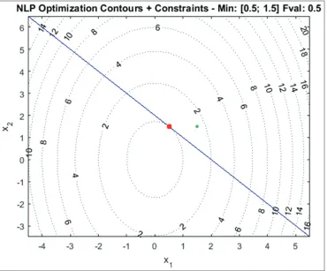
Example:Let us consider the following problem Min f x =1

2 x + 1 3x

x 1

2 22

∈ℜ

( )

 

 

2

Subject to, g(x); x₁+x₂−2 = 0

Then, the augmented Lagrangian is given by

LA x k k x x k x x x x

k

;λ µ, λ

µ

(

)

=  +   +

(

+ −

)

+

(

+ −

)

1 2 1 3 2 1 2 2

12 22 1 2 1 2

2

Hence, the minimization of L_A (x; λ_k, µ_k) yields

x _k k k x

k k k k k 1 2 2 4 3 2 4

( )

= − +

( )

= −

(

)

+ λ µ µ λ µ µ ,

The optimal solution is x* = (0.5, 1.5) and the Lagrange multipliers λ* = −0.5. Now, λ λ

µ λ

k k

k k k

x x and

+1= + _

(

12 + 22 −

)

_ 0= 1

2 , 0

3. Result and Discussions

We use the method of multipliers as an approach for solving NLP problems using augmented Lagrangian penalty function. Consider the problem (P) subject to the equality constraints g_i(x) = 0 for i∈I, the condition (2*) can be written as the function of augmented Lagrangian function because the first two terms, which are called Lagragian and are augmented with the third term associated with penalty parameter. The optimum value of λ or µ is not known in advance, so we need to build up an iteration process to find the optimum value of multipliers and we can obtain the original value of the problem. The augmented Lagrangian function has a good property that it is an exact penalty function if λ is the Lagrange multiplier at the solution if the penalty parameter is sufficiently large. For this nice property, the ALM generates a sequence of points {x_k, k=1,2…}, each of them is an approximate solution of (7). In this paper, we present the following ALM algorithm [7].

Algorithm 1.1

Step 1: Given with the iteration counter k = 0, maximum constraint violation V_maxL = ∞. Set initial val -ues for multipliers _i1, penalty parameter µ_k, penalty increasing constant c, and convergence rate α. Step 2: Estimate the initial values x0 _{for generating initial values.}

Step 3: Set k = k+1;

Step 4: Minimize the equation (2.2) and get the solution x_k*.

Step 5: Evaluate constraints g x_i

( )

*_k . Set the maximum constraint violation as

V g x

i i i

k

max=max max max

{

(

( )

,−λ

)

}

and find the set I=

{

i: max

(

g xi

( )

,−λik

)

>VmaxL/α

}

. Moreover, it is composed of many constraints that are not reduced with α.

Step 6: To check the stop criteria. If V_max≤ε, then stop; x_k* is the solution. If V_max>ε, then go to next step.

Step 7: If the maximum constraint violation in this step is larger than the previous step, i.e. V_max≥V_maxL, updating penalty factor with µ_i = c.µi for i∈I so that the Lagrange multipliers are unchanged and the value of λ_i is updated. After this updating, the iteration goes back to step 4.

Step 8: If V_max<V_maxL, then the updating λ_i as follows: λiK+1=λik+max

(

g xi

( )

,−λki

)

K 1 k i i h(x)

λ = λ + _.

Step 9: V_max<V_maxL/α, setting V_max = V_maxL, go to step 3.

Step 10: Setting µ_i = c.µ_i, λki+1=λik+1/c for i∈I, Vmax = VmaxL, and go to step 3.

However, according to Fletcher (1987) [6], step 4 to step 7 will not repeat endlessly and for sufficiently large penalty parameter.

3.1. Optimum design problem

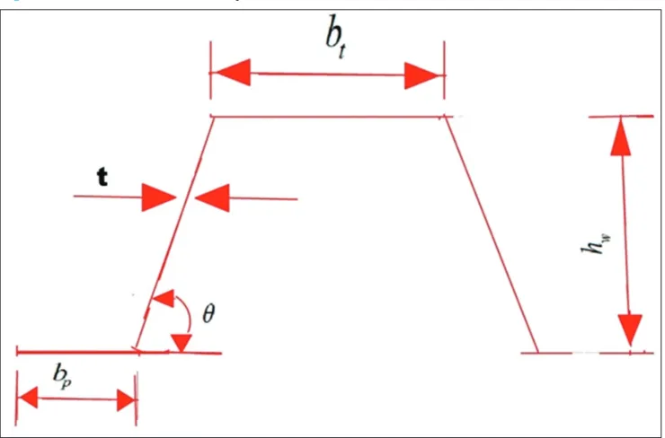
In this section, we discuss an optimum design problem following [7]. In the first section, the NLP problem (P) has many local minima in the feasible region. This class of optimization problems arises frequently in engineering optimization, especially for large-scale problems. Using the above-mentioned ALA, we can calculate the minimum weight design of cold-formed hat profile beam. We can test the design problem to show the ability of the algorithm. For this reason, we need to choose certain parameters in the above algorithm. The steel beam will be considered to be continuous over two spans in which the span length is of 4 m we will take the beam in such a way that the lateral torsion buckling will not occur. The yield strength of the steel beam is 350 N/mm2_{, the elastic modulus is 210,000 N/} mm2_{, and the density is 7850 kg/m}3_{. Let us consider the characteristic value of permanent load is} g = 1 kN/m, and variable load is q = 5 kN/m. All the loading are according to [8], and in each case, the thickness of the profile is 2 mm. The shape of this steel beam is shown in the following Figures 1 and 2.

The minimum weight design of the beam can written as follows:

Min. W = ρ.A_g (23)

Subject to the some constraints. Here, W is the weight of the beam (kg−1_{) and A}

g is the area of the beam profile which depends on dimension. We can take the design variables and introduced as the width of upper flange, the width of bottom flange and the height of the web, the inclined angle of this is and the thickness of the profile, as shown in the following Figure 3.

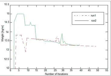
According to (ENV 1993 Euro code 3) [9], the constraints can be classified as follows: Geometrical, strength, and deflection constraints, we follow [7] to assume those types of constraints. Now, we take the design variable which is the width of the top flange b_t, which is varied from 20 mm to 200 mm, the bottom flange b_p is varied from 20 mm to 200 mm, the height of the web h_w is varied from 20 mm to 170 mm, and the inclined angle θ is varied between 45° and 90°. When running the algorithm, the population size is set to at least twice of the length of the individual string. According to Belegundu and Arora (1984), we take the initial value λ1_{i as zero and the convergence rate α = 0, and we take three different values of µ}

0 = 10,

50, and 100 and the corresponding convergence is shown in the following Figure 4.

In Figure 4, we observe that the convergence is beginning at µ₀ = 10 and fluctuating but converges later to the optimum value to µ₀ = 50 and 100. From this comparison, we conclude that this is one of the main properties of ALM, so performing extensive numerical experiment is not necessary to find specific value for penalty factor. We set the value µ₀ = 50.

4. Conclusion

From the above preliminary result, we observe that the optimal design of steel beam can be constructed with a suitable penalty function with neither small nor large penalty factor and this is the main point for the convergence. The proposed ALA is able to effectively solve the constraint problem till optimality and seems to be competitive with the so-called penalty based algorithm. Many practical engineering problems, for example, [7] and other complicated and related problems also can be solved in the near

Figure 2: The loadings on two span of the steel beam

future. From the above, we conclude that to ensure the standard optimum dimensions under certain loads for different span lengths for various practical applications, many calculations are required.

References

Adel, H., Cheng, N.T. (1993), Integrated genetic algorithm for optimization of space structures. Journal of Aerospace Engineering, 6(4), 315-328.

Bazaraa, M.S., Sherali, H.D., Shetty, C.M. (1993), Nonlinear Programming: Theory and Algorithms. Hoboken: John Wiley & Sons, Inc.

Belegundu, A.D., Arora, J.S. (1984), A computational study of transformation methods for Optimal Design. AIAA Journal, 22(4), 535-542.

Bertsekas, D.P. (1982), Constrained Optimization and Lagrange Multiplier Methods. 1st _{ed. U.S.A: Academic Press.} CEN. (1994), ENV 1991-1 Eurocode 1: Basis Design and Actions on Structers, Part 1: Basis Design.

ENV 1993 Euro Code 3: Design of Steel Structures. (1996), Part 1.3: General Rules. Supplementary Rules for Cold formed Thin Gauge Members and Sheeting.

Fletcher, R. (1975), An ideal penalty function for constraint optimization. Journal of the Institute of Mathematics Optimization, 15, 319-342.

Fletcher, R. (1987), Practical Methods of Optimization. 2nd _{ed. Hoboken, New Jersey: John Wiley and Sons.} p277-295.

Hestenes, M.R. (1969), Multiplier and gradient methods. Journal of Optimization Theory and Applications, 4, 303-320.

Luenberger, D. G., “An Approach to Nonlinear Programming,” Journal of Optimization Theory and Applications, 11, pp.219-227, 1973.

Polak, E. (1997), Optimization: Algorithms and consistent approximations. No. 124 in Applied Mathematical Sciences. New York: Springer.

Powell, M.J.D. (1969), In: Optimization, R.F., editor. A Method for Nonlinear Constraints in Minimization Problems. London, UK: Academic Press; p283-298.

Rockafellar, R.T. (1993), Lagrange multipliers and optimality. SIAM Review, 35, 183-238.