International Doctorate School in Information and Communication Technologies
DISI - University of Trento
U
LTRA
-
LOW
-
POWER
VISION SYSTEMS FOR WIRELESS APPLICATIONS
Nicola Cottini
Advisor:
Custom CMOS vision sensors could offer large opportunities for ultra-low power
applications, introducing novel visual computation paradigms, aimed at closing the
large gap between vision technology and energy-autonomous sensory systems.
Energy-aware vision could offer new opportunities to all those applications, such as
security, safety, environmental monitoring and many others, where communication
infrastructures and power supply are not available or too expensive to be provided,
This thesis aims at demonstrating this concept, exploiting the potential of an
energy-aware vision sensor, developed at FBK, that extracts the spatial contrast and delivers
compressed data. As a case study, a custom stereo-vision algorithm has been
developed, taking advantage of the sensor characteristics, targeted to a lower
complexity and reduced memory with respect to a standard stereo-vision processing.
Under specific conditions, the proposed approach has proven to be very promising,
although much work has still to be done both at sensor and at processing levels.The
last part of this thesis is focused on the improvement of the custom sensor. A novel
vision sensor architecture has been developed, which is based on a proprietary
algorithm, developed by a partner of FBK and targeted to surveillance applications.
The algorithm is based on adaptive temporal contrast extraction and is very suitable
to be implemented at chip level. Although the output of the algorithm has strong
similarities with the spatial contrast vision sensor, it relies on temporal contrast rather
than spatial one, which is much more robust for event detection applications. A first
prototype of ultra-low power adaptive temporal contrast vision sensor has been
developed and tested.
Keywords
Contents
1. INTRODUCTION ... 1
2. STATE OF THE ART ... 5
2.1.SYSTEM ... 6
2.2.VISION SENSORS ... 14
3. LOW POWER VISION SENSORS AT FBK ... 25
3.1.SPATIAL CONTRAST SENSOR ... 26
3.2.TEMPORAL CONTRAST VISION SENSOR ... 34
4. CUSTOM STEREO VISION SYSTEM ... 39
4.1.CUSTOM STEREO ALGORITHM ... 40
4.2.STEREO VISION SYSTEM SIMULATION ... 50
4.3.SYSTEM SPECIFICATIONS AN REALIZATION ... 51
4.4.EXPERIMENTAL RESULTS ... 61
4.5.CLOSING REMARKS ... 67
5. ULTRA LOW POWER VISION SYSTEM FOR SCENE INTERPRETATION... 68
5.1.CUSTOM CHIP EMBEDDED ALGORITHM FOR SCENE INTERPRETATION ... 70
5.2.ALGORITHM SIMULATION ... 74
5.3.SYSTEM REALIZATIONS ... 78
5.4.SYSTEM RESULTS ... 81
5.5.CLOSING REMARKS ... 84
6. CONCLUSIONS ... 85
List of Figures
Figure 1. Simplified block diagram of a standard sensor processing system,
including: sening, digital processing and communication. ... 3
Figure 2. Simplified block diagram of a custom sensor processing system, including: digital sening, digital processing with active feedback for sensor and communication. ... 3
Figure 3. Panoptes, smart camera mote architecture hardware and power consumption... 7
Figure 4. Mesheye, energy-efficient smart camera mote architecture. ... 8
Figure 5. Meerkats Power-aware, Self-Managing Wireless camera network for Wide Area Monitoring. and Power consumption ... 8
Figure 6. Cyclops couples with a Berkeley Mote and they represent a wireless vision network node. ... 9
Figure 7. Visual sensor node for Bluetooth-Based Measurement Networks. ... 10
Figure 8. Bio-inspired vision node based on address-event image approach. ... 11
Figure 9. Architecture of the Anafocus Eye-RIS system. ... 12
Figure 10. Eye-RIS v1.3 and v2.1 vision system. ... 13
Figure 11. Dynamic scene taken by Tobi Delbruck’s sensor ... 18
Figure 12. Sampled intensity from the Temporal difference about Etienne-Cummings sensor. ... 18
Figure 14. Lichtsteiner’s output, where the two people are moving to opposite direction . The leading edges produce OFF spikes and trailing edges produce on spikes. 19
Figure 15. Bio-inspired vision sensor developed by FBK ... 20
Figure 16. Rüedi’s sensor, contrast kernel, masch, contrast representation ... 21
Figure 17. Kim’s sensor and Edge detection algorithm using WTA and LTA functions. 22 Figure 18. Example two different imges extraction techniques (a) Motion detection by frame difference and (b) full kernel edge detection ... 22
Figure 19. Example of a moving object acquired by the sensor working in (a) normal contrast mode; and (b) in motion extraction mode. ... 23
Table 2. Characteristics of the custom vision sensors presented. ... 23
Figure 20. (a) 3x3 Kernel of standard filter, (b) Kernel of three adjacent pixel of sensor used. 27 Figure 21. Simulation of the spatial contrast algorithm implemented in FBK sensor. 28 Figure 22. Schematic of the pixel-level contrast extraction circuit. ... 29
Figure 23. Shows a timing diagram of a frame acquisition. ... 30
Figure 24. Block Diagram of the Spatial contrast sensor. ... 31
Figure 25. Example of data coding and temporal input output signalas. ... 33
Figure 26. Portion image, data coding and memory rappresentiation. ... 33
Figure 27. Conventional low pass filter. Figure 25. Equivalent low pass filter with switched capacitor. ... 35
Figure 28. Pixel schematic of temporal contrast sensor. ... 36
Figure 29. Temporal sequence of object absorption. ... 37
Figure 32. Top vision from the pattern of cameras and differente disparity proiection. 42
Figure 33. Sensor image date deliver in spars matrices organization. ... 44
Figure 34. The pair of images left and right respectively e the ideal result the disparity algorithm are represented. ... 44
Figure 35. In vertical line we represented a row of left image end in horizontal we represented the same row delivered by the right sensor. ... 45
Figure 36. Two corrispondent row and the disparity. ... 47
Figure 37. Example of cost function constraint. ... 49
Figure 38. Simulationa results a)Left binary image b)Right binary image c)Real scene d)Disparity resoults. ... 51
Figure 39. Top vision from the pattern of cameras. ... 52
Figure 40. Top vision from the pattern of cameras. ... 53
Figure 41. Laboratory Stereo vision simulation. ... 55
Figure 42. This picture represents left and right vision extracted by the same camera. 55 Figure 43. First Stereo prototype ... 56
Figure 44. a) First prototype, b) Block diagram, c) GUI. ... 57
Figure 45. Calibration scene ... 58
Figure 46. Different projection of the Calibration process. ... 59
Figure 47. Rectifications resolut. ... 60
Figure 48. Prototype of the overhead people counting system. In the blow-up, the stereovision system is depicted with geometric details. ... 61
Figure 49. Example of the disparity maps obtained. a) Identification of Heads, Shoulders and Feet b) Body and shadow discrimination c) Identification of different heads 62 Figure 50. Depth resolution of stereo vision system realized. ... 63
Table 4. Number of operations comparison (ops) , general case full block Matching,
Philipp and ... 65
Cummings hardware implementation and this algorthm. ... 65
Figure 52. Real images and output of feature extraction algorithm ... 71
Figure 53. Funcitionality pixel algorthm ... 75
Figure 54. Output of pixel algorthm.Green rappresent the QMax and yellow the QMin 77 Figure 55. Prelinary funcitionality pixel test with pattern generator ... 78
Figure 56. Evaluation parameter of the transfer function a) step-up b) step-down 79 Figure 57. The prototype realized on FPGA platform usb link with a PC ... 80
Figure 58. First measure of real benchmark movie. ... 81
Figure 59. Labview interface. On top Vp,Vmin e Vmax abalog values are ripectivly rapprest. At the bottom Digital imgage changes,min memory changes, max memory changes ... 82
Chapter 1
1. Introduction
high-performance computing platforms. The natural way obtaining information of the world around us is visual. We obtain more than 90% of information about the world surrounding us with our eyes, and about half of our brain is busy with its interpretation. Even small animals, birds and insects can easily interpret the visual world surrounding them - this with a fraction of the computational power of an ordinary computer. On the other hand, an artificial vision system is a system that observes the visual world around it and interprets it to provide information about the scene. Such systems are currently bulky, expensive, power hungry, and instead of having cognitive capabilities are often limited to image recording. They are widely used in surveillance and security systems, traffic and pedestrian monitoring, etc., which require infrastructures for the power supply and data communication. They all are based on standard electronic hardware, which is not specifically optimized for energy-aware operations. For example, a commercial imager continuously delivers sequences of images with large redundancy becouse only a small amount of the available information is used to perform a visual task. The processor is required to execute visual processing even though no relevant information occurs in the scene, turning into a large waste of power and of computing resources. These aspects are of main importance in case of a long lasting autonomous system, which has to operate with a limited available energy budget. Although microelectronic technology has brought significant improvements in system performance and energy efficiency, vision computation did not make over the years significant progress in energy-autonomous applications in recent years. While the power consumption of a standard vision system can range from a few Watts to tens of Watts, a wireless sensor node burns typically mW on average. This means that there is a gap of 2 to 3 orders of magnitude in power consumption between these two technologies.
Figure 1. Simplified block diagram of a standard sensor processing system, including: sening, digital processing and communication.
As shown in ( Figure 1. ), the signal provided by the sensor is firstly converted into a digital form by the A/D converter, feeding the digital processor for . The output of the signal processing unit is sent to a PC or a base-station through a wired or wireless link. Here, each functional block is intended to execute a specific operation with the required performance, but has only limited interaction with the neighboring blocks. Therefore, the energy efficiency does not only depend on the performance of each single block, but it also relates to the cooperation among the different units of the system. System-level design has indeed a large impact on the energy consumption. At a first glance, embedding some programmable intelligence at sensor level, making it able to recognize and extract significant features in the scene, would drastically increase the energy efficiency of the system, without losing performance. Although, the main benefit of doing this is a reduction of redundant data, thus less data to be processed, an adaptive system would be more desirable, making it to modify its operating functions according with the specific scenarios and with the available energy. In other words, the energy management concept needs to be applied at system-level in addition to each single block of the signal path.
Figure 2. Simplified block diagram of a custom sensor processing system, including: digital
sening, digital processing with active feedback for sensor and communication.
Sensing Digital processor Transceive r
Algorithms for visual processing will also play a key role in the system design. As always, algorithms are severely limited by the hardware and have to be tailored to exploit the potential of the current system architecture.
CMOS technology allows the integration of image sensing with massive parallel visual processing architectures, where the custom vision sensor can be dynamically programmed though a feedback of second level algorithm ( Figure 2. ). This approach offer a unique opportunity of introducing novel energy-aware computational paradigms, closing the gap between vision technology and energy-autonomous systems.
This thesis aims to deal with the energy-aware visual computation issue by exploiting the potentials of two custom low-power vision sensors, combined with lightweight algorithms, based on event-detection and are targeted to monitoring applications. Novel processing paradigms has been investigated, aimed at optimizing the senor custom data coding with minimum use of memory and computing resources. Two, proof-of-concept demonstrators has been developed, demonstrating the validity of the proposed approach.
Chapter 2
2. State of the Art
Since last decade, a lot of effort has been spent by the research community in bringing vision systems into the battery-powered category, by using Components Off The Shelf (COTS). This has brought to the development of some vision prototypes performing relatively simple event detection operations with hundreds of Watts to few Watts of power consumption. This hampers those systems to be used for long-lasting operation powered with batteries.
2.1.
System
Most of the groups that develop CMOS imagers today perform image processing on frame-based hardware [1][2][3][4][5][6][7][8]; this means that the image is acquired during exposition time and dispatched to the output of the device, pixel after pixel, sequentially, in a raster-scan fashion. In most cases, this is the only feasible approach, driven by the market availability of the imager technology.
Commercial imagers (Components Off the Shelf: COTS) operate on frames. Acquisition of frames and processing them dominates the power consumption of existing demonstrations.
In the field of wireless sensors networks, several video sensor nodes have been reported, which are connection points of a network capable of sending, receiving, or forwarding information over the communications channel. All these system are based on COTS to meet the tight cost constraints typical of distributed sensing applications. For example, Panoptes [9] developed in 2003 by Feng et al. at the OGI school o Science of Portland State University and subsequently improved at the Department of Computer Science of Portland State University.
The prototype is equipped with an Intel StrongARM processor, a Logitech 3000 camera and Linux OS. Its power consumption is more than 5W Figure 3. Delivering the stream of image at 20 fps with a resolution of 320 x 240 Pixels. The new prototype adopt the Crossbow Stargate Platform decreasing power consumption at 4W.
To supply solar power to this device, a solar panel of about 2 sq. meters and a car-sized supporting battery would be required.
Figure 3. Panoptes, smart camera mote architecture hardware and power consumption
Another example of a visual sensor is the MeshEye [10] (Figure 4. which has much lower power consumption. Although a benchmark has to be considered to properly evaluate the performance of the system, this smart camera is claimed to last about 22 days with 2 AA batteries (less than 2 fps). This system is intended to work in periodic poll intervals, where the microcontroller wakes up periodically, acquires an image and determines if something has entered the scene. Once an object has been detected, intermediate level processing extracts its descriptive representation. MeshEye is capable of detecting, acquiring and tracking objects entering the scene, thus it is suitable for surveillance applications.
Figure 4. Mesheye, energy-efficient smart camera mote architecture.
This system incorporates 2 1k-pixel imagers (optical mice sensors) and 1 VGA resolution image sensor with a microcontroller and Zigbee wireless radio interface. The philosophy of this system consist to use the low level imager to detect the basic movement preset in the scene and when a movement are detected the second level imager is wakeup.
Figure 5. Meerkats Power-aware, Self-Managing Wireless camera network for Wide Area
Meerkats [11] (Figure 5. belongs o the same class of Panoptes, but uses more recent components (XScale processor). The goal of this work is Process an image before transmission, cut off a region involved by event, and extracting features such as motion flow, may decrease the amount of data being transmitted.
Figure 6. Cyclops couples with a Berkeley Mote and they represent a wireless vision network
node.
Cyclops (Figure 6. is a much lower power device, making use of Xilinx CPLD and Atmel microcontroller ATmega128L and a sensor with a CIF resolution (352×288) [12]. It achieves less than 4 fps for basic (presence/absence) object detection task on small images (128 x 128 pixels).
Power Consumption: a) stand-by < 50μA; b) 5mA@4MHz clock freq.; c) 11mA@13MHz clock freq.
Figure 7. Visual sensor node for Bluetooth-Based Measurement Networks.
In a surveillance application, the sensor may send alert images for verification to security personnel only when the sensor identifies an alert condition. In monitoring applications (people counting, traffic monitoring) no images may be sent, only small data packets requiring a minimal bandwidth and minimal power for transmission. In contrast with standard systems, would not be necessary to deliver continuously stream video information. Ideally, triggers on significant events in the scene, extract features, and dispatch only this information, to permit drastically cutting down the bandwidth and of course energy consumption.
In order to do this is necessary to understand where removing the most irrelevant and redundant features from the data in efficient way. The most efficient way to extract the important information present in the scene it’s execute this pre elaboration directly on chip avoiding an overload of data to other elaboration blocks. This approach require custom sensors, because in general the sensors are not able to deal with events.
The AER is a communication protocol in frequency. The information is encoded by the intervals of time inter spike (ISI, Inter Spike Interval). The pixels used in this retina allow to best use the capacity of channel. Only the pixels that have something to communicate requesting to external bus access. Completely different situation respect to a raster used by conventional sensors. The sequence of spikes that travel along the external bus are only those from the pixels that show variations in light intensity. The pixels of the matrix are completely independent and no busy signal is communicated to the various neurons in the case where one of them is issuing the spike, their loading the external bus with a identifies code (x, y locations). A selection system between neurons in the competition for access to the bus is necessary. The circuit part which operates this selection is called the arbiter. The arbitrator chooses which neurons give access to the bus AER depending on the timing for submission of requests access.
Figure 8. Bio-inspired vision node based on address-event image approach.
VGA camera, OmniVision OV7649, interfaced with a XScale processor (PXA271). As wireless node, an Intel iMote2 has been adopted. Working in full active mode at 104MHz and 8fps, the entire system consumes 322mW in which the iMote2 is responsible of 279mW.
The Anafocus Eye-RIS [15] is an interesting example of vision systems on the market, which is based on a custom vision chip [16]. The Vision System on-Chip (VsoC) architecture (Figure 9. ) performs image processing at three different levels:
1 : pixel-level processing, in which each pixel includes analogue and binary processor and memory.
2 : column-level processing which represents a linear array processor able to readout and cooperate to process one or several image rows as required by the algorithm.
3 : system-level processing is a powerful on-chip microprocessor designed to speed-up power consuming task.
Figure 9. Architecture of the Anafocus Eye-RIS system.
Image pre-processing targets extracting useful information from the input image flow; this means eliminating all redundant, and therefore useless, information for the specific algorithm being accomplished. It consists of relatively simple processing tasks, such as image convolutions, spatial filtering, morphological and statistic operations; combined in algorithms that are intensively applied to each captured image. Image post-processing targets making complex decisions and supporting action-taking. It normally involves complex algorithms within long and involved computational flows and may require larger accuracy than early processing. The major benefit introduced by this architecture is the reduction of on-chip memory and overall system power consumption.
Figure 10. Eye-RIS v1.3 and v2.1 vision system.
The Eye-RIS v1.3 (Figure 10. ) vision system has a resolution of 176x144 pixels and performs high performance image acquisition at high speed (over 10000 fps) with mixed-signal image processing with fast electronic global shutter characteristic, showing a typical power consumption of 1.5W.
The multiple board architecture and reconfigurable FPGA allows the system high flexibility, permitting its easy adaptation to the requirements of specific applications, but these approach introduce some limitations in term of power consumption.
The last two works demonstrate the importance to optimize all parts of the system, but especially the vision sensor. In fact it is just the sensor to determines the type and the quantity of date will be processed. It therefore becomes necessary to analyze the state of the art of custom sensors.
2.2.
Vision sensors
Current commercial imagers are almost always designed for multimedia applications - mobile phones, digital video cameras and toys, where low cost and high image resolution are the main figures of merit. CMOS has almost replaced CCD technology in the imagers scenario, at least for the consumer market. The big advantage of CMOS image sensors over the traditional CCD sensors is in their capability of integrating sensors, A/D conversion, digital signal processing, such as auto exposure control, pixel correction, face-smile detection etc., in a true System On Chip paradigm.
On the other hand, CMOS offered the possibility of developing novel architectures and un-conventional approaches for image sensors, which are more oriented toward custom and special applications requiring sensors with advanced performance.
Among others, low power performance is going to become a priority. This is because mobile devices are almost ubiquitous as well as sensors is the technology which promises to drive the semiconductor market for the next decade.
With such common architectures, sensor power consumption is secondary to that of the overall system: DSP, memory and communication unit. All this results in high power consumption. For example, a 70mW commercial VGA CMOS imager is claimed to be an ultra-low power sensor. Powered with a small 950mAh Li-ion battery, the imager can only run for 38 hours, without taking into account additional system components, which are usually much more power hungry than the sensor itself. This gives us a rough estimation of the lifetime for a battery-operated vision system, based on commercial components, even in the most optimistic scenario. Several tentative battery-powered vision systems, based on Commercial-Off-The-Shelf (COTS) components, have been produced in the last decade. They did not obtain encouraging results in terms of operating lifetime, due to their large power consumption, ranging from hundred mW up to several Watts. On the contrary, they proved that the custom design is definitely the best approach for developing low-energy vision systems.
In the literature, several examples of custom vision chip implementations are reported, aimed at low-power applications. While interesting, the majority typically confront only the sensor perspective, without taking into account other important system-level issues: high-level image processing, data communication and energy management. Specification Kagawa[17] Gottardi[18] Fu[19] Hanson[20] K.Cho[21] Tang[22] Law[23] Cmos Technology 0.35µm 0.35µm 0.5µm 0.13µm 0.13µm 0.35µm 0.35µm Number of Pixel 128x96 128x64 64x64 128x128 128x128 128x96 32x32
Fill Factor 18.5 20 23 32 38 39 21
Frame Rate 9.6fps Up to4000fps 60 fps 8.5 fps 15 fps 9.6 fps 21 fps Supply Voltage 1.35V 3.3V 3V 0.7V 1.25V 1.35V 1.5V Total Power 55µ[email protected] 20µW@10fps 1.2mW 0.7µ[email protected] N/A 55µW@10fps N/A Consumption 460pW/fr.pix 269pW/fr.pix 4.9nW/fr.pix 85pW/fr.pix N/A 460pW/fr.pix 821pW/fr.pix
Interestingly, very advanced performance is claimed. However, it is worthwhile to analyze carefully the architectures reported. This is not always a simple task. In fact, the presented implementations are very different from each other (pixel topology, ADC, chip interface, subsequent processing). Moreover, the data presented on power consumption is not homogeneous: total power, power/pixel, power/array, power/ADC conversion, etc. Although no standard has been defined yet to enable rigorous comparison between the implementations, a good figure of merit is the power consumption per frame per pixel (W/frame.pixel). This value includes the actual consumption of the pixel together with a share of consumption of the sensing circuit, A/D conversion and chip interface.
State-of-the-art CMOS imagers exhibit pixel size of 1,4μm x 1,4μm and 8 Mega-pixel resolution [24].
Recent trends toward wireless sensor networks necessitate an efficient way to extract visual data from a camera meeting the limited energy budget of the sensor node. Conventional scanned imagers are not able to fulfill these requirements due to their poor efficiency in the use of the signal bandwidth and the requirement for expensive video processing on the raw pixel data.
This approach was taken by Teixeira et al. [25] at Yale University, New Haven, CT, USA. Their work proposes a non-standard imager in which the concept of frame is replaced by an Address Event Representation (AER).
The (AER[26][27][28]) has been demonstrated to be an efficient method to communicate information among bio-inspired subsystems, especially for vision chips. Several implementations have been reported in the literature [29][30][31]. AER systems are based on spikes generated by those pixels reaching threshold. The pixel generating a pulse asks the system to be read out. The communicating system is asynchronous and assigns resources only on demand, resulting in better energy efficiency than traditional synchronous systems, which allocates the same bandwidth to all the pixels of the array. A reported 64 x 64 pixel image sensor adopts the AER architecture with a low power consumption of 5.75μW and a dynamic range of 235 dB [32]. Even though very wide dynamic range has been demonstrated, the imager is not intended to perform image preprocessing.
In literature, several examples of vision sensors implementations are reported, targeted to low power applications. Even though most of them represent interesting implementations, the majority approaches the problem from the sensor perspective, without taking into account the system-level data communication and energy issues [33][34][35][36].
In fact, almost all the developed vision sensors are more concerned about performance rather than performance/power consumption.
Temporal gradient
The vision sensor present by Tobi Delbruck [37] adopt the AER approach where the output consists of asynchronous address-events that signal scene reflectance changes at the times they occur. This sensor is inspired to biological retina principle. The figure Figure 11. represent the output of the sensor it possible to show the efficient filter able to remove the background activity, this permit only the movement extraction.
The sensor is characterized by 128x128 Pixel by it has 40 x 40 μm2 pixels with 9.4%
fill factor, the Dynamic range is 120 dB and chip power consumption is 23 mW.
Figure 11. Dynamic scene taken by Tobi Delbruck’s sensor
Other publication are focused on power consumption, Dongsoo Kim [39] declare 1 mW with a 3-V of power in active state where the sensor it is able to compute the temporal difference between continuous frames and filter out redundant data.
The sensors is caraterized by 64x64 pixel it has Each pixel occupies an area of 29 × 28 μm2 with a fill factor of 23%.
Figure 13. Dongsoo Kim Image sensor, test board and measured results with the human
movements.
The sensors realized by P. Lichtsteiner and T. Delbruck [40] reduces image redundancy by responding only to temporal changes in log intensity. Where Static scenes produce no output. Image motion produces spike event output that represents the changes in image intensity. It has 64x64 pixels Each (40um2) the fill factor (8.1%) where the power consumption is 7mW.
Figure 14. Lichtsteiner’s output, where the two people are moving to opposite direction . The
Not all custom sensors are based on a temporal different but an alternative it’s the spatial gradient extraction.
The 64x64 bio-inspired pixels vision sensor developed by FBK with adaptive dynamic background subtraction the sensor detecting temporal changes in light intensity between two successive frames in binary form.
This sensor can dynamically adapt to changing scenes, in order to compensate for slow-varying levels of illumination and detect the high-varying. This sensibility can be tuned by the external control. We will see better this chip in the next chapter.
Figure 15. Bio-inspired vision sensor developed by FBK
Other types of elaboration can be Implemented on-chip one of this are the spatial filter, are used for feature extraction such as edge detection.
Below we report some spatial gradient implemented on chip present in literature.
Spatial gradients
The chip dispatch information by decreasing order of contrast magnitude obtaining two main advantages first all the significant information is delivered first and the amount of data dispatched out of the circuit can be tuned for different task. But the relevant number of operation inside the pixel increase the pixel size is 69x 69 µm2 and reduce a fill factor of 9%.
Figure 16. Rüedi’s sensor, contrast kernel, masch, contrast representation
Another example is the sensors developed by Dongsoo Kim [42] characterized by pixel area is 16×21 µm2 and the power consumption performance is not very low power, is 1.2 mW at 3 V .
The 128 ×128 smart pixel array extract intensity, spatial contrast, and temporal difference images. The spatial contrast, where the pixel (i,j) finds the maximum and the minimum photo-integrated signals with the winner-takes-all (WTA) and loser-takes-all (LTA) in the 4 adjacent pixels {(i,j),(i+1,j),(i,j+1),(i+1,j+1)}.
Figure 17. Kim’s sensor and Edge detection algorithm using WTA and LTAfunctions.
Spatio-temporal gradient
The vision sensor designed by Massari [43] consists of a 128x64 pixel array. The pixel-parallel vision sensor architecture that offers higher flexibility where novelty of the approach consists in its capacity to acquire images with a dynamic range up to about 100 dB, combining pulse-based and time-based signal processing technique, during the integration phase. The main characteristic is a highly programmable vision architecture, able to implement a different class of pixel-level spatio-temporal filtering. Spatial contrast are executed with full 3x3 pixel kernel connectivity and temporal contrast for motion detection is implemented by two successive frames difference.
Gottardi [18] propose a 100 µW 128 x 64 Pixels Contrast-Based Asynchronous Binary Vision Sensor for Sensor Networks Applications. It’s a ultra-low power 128 x 64 pixels vision sensor, characterized by pixel-level spatial contrast end temporal contrast extraction and binarization.
(a) (b)
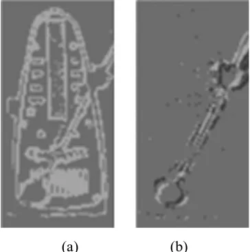
Figure 19. Example of a moving object acquired by the sensor working in (a) normal contrast
mode; and (b) in motion extraction mode.
Resolution Pixel μm2 Fill factor Dynamic range Power
Tobi Delbruck 128 × 128 40 × 40 9.4% 120 dB 23mW
Etienne-Cummings 189 × 182 25 × 25 30% 30mW at 50 fps from 5V
Dongsoo Kim 64 × 64 29 × 28 23% 1 mW a 3-V
P. Lichtsteiner 64 × 64 40 × 40 8.1% 7mW
FBK temporal contrast 64 × 64 30 × 30 12% 620pW/frame*pixel
Rüedi 128 × 128 69 × 69 9% 120dB 300 mW 3.3V
Dongsoo Kim 128 × 128 16 × 21 42% 1.2 mW 3 V
Massari 128 × 64 32.6 × 32.6 24% 14 mW 3.3V
Gottardi 128 × 64 26 × 26.5 20% 100dB 100uW 3.3V
Chapter 3
3. Low power vision sensors at FBK
As mentioned in the previous chapter, the custom sensors are powerful candidates for energy-aware applications. Both embed custom visual processing algorithms at pixel-level with low power consumption/pixel together with pixel-pixel-level A/D conversion. Custom data coding and compression has been adopted to avoid redundancy and minimize the activity at the sensor interface.
One of the objectives of this PhD is focused to the exploitation of these two vision sensors developed at the Fondazione Bruno Kessler (Trento) and targeted to low power applications. This activity relates to the development of the electronic systems, the conception and design of novel image processing algorithms, taking advantages from the custom image processing.
FBK institute designed different type of sensor based on two different approaches: - Spatial contrast extraction
- Temporal contrast extraction
intended for definition as the ratio between the brightness difference of the two areas and their sum also defined as the Michelson:
ΔI= min max min max I I I I
Often, the information is dispatched following the intensity map criterion, which is not a good representation for detecting salient features from a scene. Even though the sensor has very low-power consumption, it is not able to directly trigger salient events of the scene. Image processing is demanded outside the chip.
Another sensor develop on FBK institute is based on the temporal contrast.
The Temporal contrast is the ability to detect variations in luminance over time, is required for motion extraction.
If consider a intensity value Iij to a pixel, it can be represented as: ΔIij (t)= Iij (t) – Iij (t-1)
The ΔIij represent the changes intensity value pixel by pixel from previous frame related to movement present in the scene, in order to discriminate real movement from noise most techniques work with some threshold.
3.1.
Spatial contrast sensor
One of the sensors designed by the FBK researchers Gottardi[18].This sensor directly extracts the spatial contrast of an acquired image directly on chip exploiting the Weber contrast approximation: B B I I I
The spatial contrast extraction in most robust respect the standard edge extraction because the different extracted it’s normalized. In this way the dynamic range of the signal analyzed is unconnected of this type of measurement, in fact it’s possible to map a type of disparity in priory range known. In general this algorithm are implemented using the kernel, where the comparison between the pixels are executed.
(a) (b)
Figure 20. (a) 3x3 Kernel of standard filter, (b) Kernel of three adjacent pixel of sensor used.
The dimension of this kernel it’s related of the complexity and the precision we will be obtained. The sensors for each pixel use only the different incident irradiance between a three-pixels kernel composed by, the pixel itself, the pixel on right and the pixel at its above.
The sensor at pixel-level directly extracts the spatial contrast of images in binary form through auto-adaptive technique, allowing a target to be distinguished from the surrounding background. (Figure 21.
The date delivered represent only the counter edge present in the scene, in general, in the image the pixels involved are few compared with the image resolution (15%), which guarantees the minimum I/O bandwidth.
Figure 21. Simulation of the spatial contrast algorithm implemented in FBK sensor.
This hardware implementation allows to execute the elaboration directly on chip for any pixels simultaneously increasing the efficiency in term of power consumption and speed readout. Another important innovation is the address representation of the sensor, which delivers data in a sparse-matrix through a positional coding.
In the chip the image pre-processing operations are implemented through an integrated binary frame buffer, which allows the extraction of features such as contrast, extraction of the motion and the background subtraction.
The sensor has been designed to operate in two different modes:
ACTIVE: the sensor acquires and executes a temporal matching between current and reference images, dispatching the relative address pixels to the output;
IDLE: the sensor executes the same functionality, without dispatching pixels to the output, but it provide only the number of disparity pixels present in the scene.
Pixels functionality: the architecture of a single pixel, is show in Figure 22.
It’s composed of five basic elements: the photodiode, two comparators, a block of contrast and a memory cell to one bit, together with all other, composes a matrix capable of storing a complete image.
Figure 22. Schematic of the pixel-level contrast extraction circuit.
Figure 23. Shows a timing diagram of a frame acquisition.
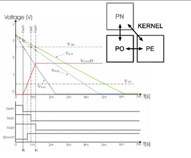
After the reset phase any pixels star a voltage discharger ramp due to the incident light. The Vpix0 is connected to contrast block with other two analog signal VPN VPE and the other three comparator (OO,ON,OE).
During this contrast estimation process the Vc is sampled and quantities regulated by this formula VEDGE0(t2) = VPO(t2) − VPN(t2).
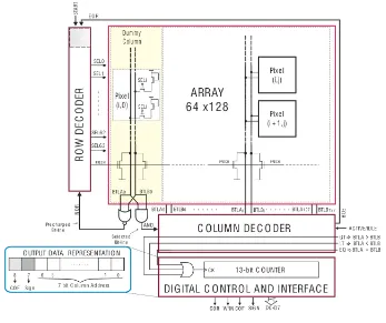
Figure 24. Block Diagram of the Spatial contrast sensor.
The internal architecture of the sensor, visible in ( Figure 24. ), comprises in addition to the matrix of pixels, also the logic required for the management of the array and output data; it has the aim to minimize the amount of control logic from added externally.
The Row-decoder select the 64 lines of the image sequence. The pixels of the row selected write two bits on the respective lines: BTLA for the current frame BTLB for the previous frame.
The Column-decoder controls the possible disparity between BTLA and BTLB in sequence and provides a pulse on one of the three bit lines (GT, EQ, LT) depending on the type of disparity, after which increments the counter.
COR is made logic high represents a newline, and passes the control to the next line. At the end of the process of image reading, then after 64 pulses of the COR, the bit of the end frames (COF) assumes high logic value and the sensor is stopped a new command are waiting to start another cycle of acquisition. The column address of the current pixel and placed at the exit asynchronously in blocks of data at 80 MB/s.
The counter to 13bit about the digital interface it’s used in different ways on the different mode closed, Active or Idle.
In Active Mode the sum of the pulses on three bit lines is always 128 number per Frame. So, putting the three-bit-lines as input to the counter clock signal, its value will be equivalent to the address column of pixels processed. When a disparity is detected, the counter value, which corresponds to the column of the pixel related, is incremented and sent out together with the sign of the disparity. Differently, if any disparities are detected, the counter is still incremented, but the data is retained, maintaining the output data very low. At each end of the row the counter is reset and the process for the Next line begins.
In Idle Mode only on the pulse of the column decoder lines that indicate a disparity (GT and LT) are considered without resetting the counter at each end of row, at the end of the scanning process of the frame the in a counter the total number of disparities present in the image will contained. During the entire raster scan of the sensor any data at output are delivered, in fact, only at the end of the acquisition phase the value stored in counter 13 bits will be delivered. The data will be divided into the upper part and lower part due to the limited number of lines.
directly the position information of the active pixels, so to permit to reduce computation and bandwidth.
Figure 25. Example of data coding and temporal input output signalas.
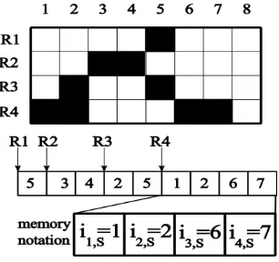
Now Considering one row of the array, for each pixel the address is delivered according with the raster-scan mode.
The Figure 26. Represent a image portion in active mode extracted an corresponding code.
Figure 26. Portion image, data coding and memory rappresentiation.
But main issues here is that binary contrast is in fact a fairly poor information, which is not reliable enough for certain applications. But vision sensor are the ultra low power characteristics in fact draws approximately 100uW at 3.3V at a frame of 50fps in a sparse-matrix through a positional coding.
The unconventional positional data coding permit to reduce the bandwidth on the other hand open problem to maintain the same efficiency on algorithm elaboration.
3.2.
Temporal contrast vision sensor
Differently the spatial contras sensors the temporal contrast sensors are based on pixel to pixel comparison between two different frame over the time. In this way only the motion events caused by the moving are delivered and automatically remove the static background.
The sensor during the integration time acquire a intensity value after that compare this value with two memory value simultaneously (SIMD). Where in this memory are keep the low values and the high reelected of low and high acquire during the previous frames.
Most of these implementation, are very sensitive to the threshold Th and works correctly only in particular conditions of object speed and frame rate.
In fact the threshold of sensor Th is modeled as an exponential moving average:
jj
j
F
Th
Th
1
1
where Fj represent the current frame and α a constant smoothing factor between 0 and 1. This peculiarity permit to adapt the sensibility of movement through the α parameter. With the aim to obtain dynamic thresholds the sensor using a low pass filter.
This architecture should be implemented pixel by pixel and it would be impossible the CMOS integration. For this reason it was necessary to find an alternative method for large scale hardware implementation.
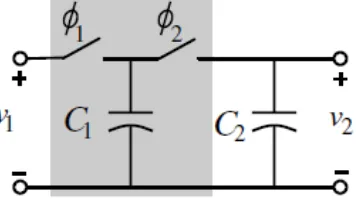
Figure 27. Conventional low pass filter. Figure 25. Equivalent low pass filter with
switched capacitor.
The method adopted is based on the equitant between the rc network and the switched capacitor.
This circuit was developed by replacing the resistor, R1, of the standard low pass filter
circuit with the parallel switched capacitor resistor circuit opportune controlled.
ck
f
C
R
1
1
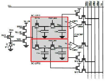
In order to understand better de characteristics of the sensor the Figure 25. Represent the hardware implementation on chip.
Figure 28. Pixel schematic of temporal contrast sensor.
The photodiode (PD) of Figure 28. works in storage mode, with a source-follower readout transistor, which is turned on by Vp clk only when necessary, reducing the pixel DC power consumption.
The two SC-LPF1/2 starting from the value VP proportional at the photodiode current extracted, evaluate the VMax and VMin values respectively for any frame rate.
In the first step the Current Vp extract by the photodiode is sampled trough the SetVp input on temporal memory C1M and C1m capacitors.
The two output of the filters are stored onto the PMOS capacitor C2M (C2m).
01
2
1
1
1
1
f
n
M
C
M
C
s
s
s
H
n
where the C1M and C2M proportional, characterize the filter characteristics.
The two output of the filters are stored onto the PMOS capacitor C2M (C2m) in order to keep of past signal variations for the next comparison .
At the end of the integration time, the CLKCOMP activated the comparators (CMP1, CMP2) and compare VP with VMax and VMin respectively stored in two analog memories, generating the two bits QMax and QMin.
Differently as previous sensor this sensors deliver all pixel value in a raster scan mode, but the binary form it’s common.
Figure 29. Temporal sequence of object absorption.
The output binary signal (QMax, QMin) delivered by each pixel are collected at the array level and can be processed outside the chip by the higher-layer algorithm trough different n value setting, implementing high level vision tasks.
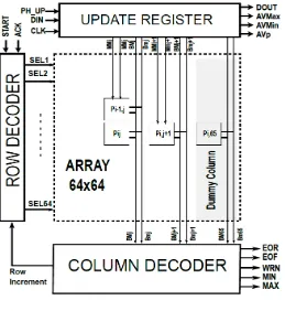
Figure 30. Block diagram of temporal difference sensor.
The Figure 30. shows the block diagram of the sensor architecture for an array of 64x64 pixels prototype. The imager is an addressable array of pixels, with a 64-cells ROW DECODER and a 64-cells COLUMN DECODER. The UPDATE REGISTER consists of a 64x2-stages shift-register with two main functions:
READOUT: after a row-selection, bit-lines are loaded into the UPDATE REGISTER and read out serially, through DOUT, CLK;
Chapter 4
4. Custom stereo vision system
We will concentrate our work on of custom sensors and custom algorithm optimization within the optimized embedded system realization. In the first part of this chapter we will analyze the principle of stereo vision and evaluate the possibility of applying this technique to a custom vision sensor with positional data coding characteristics.
The sensor has evident low power characteristics, in addition to the efficient data representation that exploits on the one side the advantages for compression and on the other side a new algorithm for elaboration phase are required.
The positional data coding eliminates the redundant information present in the image, this type of coding has all the characteristics to be exploited for images comparison. As we can see in this chapter the stereo vision is a typically complex computational technique based on the matching of portions image extracted for two different point of view. Stereo Vision System is a leader much studied considering the numerous applications in both the private and industrial, especially in the latter where applications often require three-dimensional passive monitoring devices.
matching software. Only few of them take into consideration the power consumption or the hardwire connection.
In fact, these systems are targeted to applications where high resolution and color information are of main concern.
Stereo-vision algorithms require a highly intensive signal processing based on spatial matching with large operation redundancy. In this context, the use of a custom vision sensor could have the advantage of pre-selecting the data that will take part in the processing, thus minimizing the subsequent amount of operations [18].
4.1.
Custom Stereo algorithm
If we analyze a single image is not possible to reconstruct the three dimensional structure of the observed scene. This is due to the loss of information in the perspective projection, which maps points in 3D space in a 2D space.
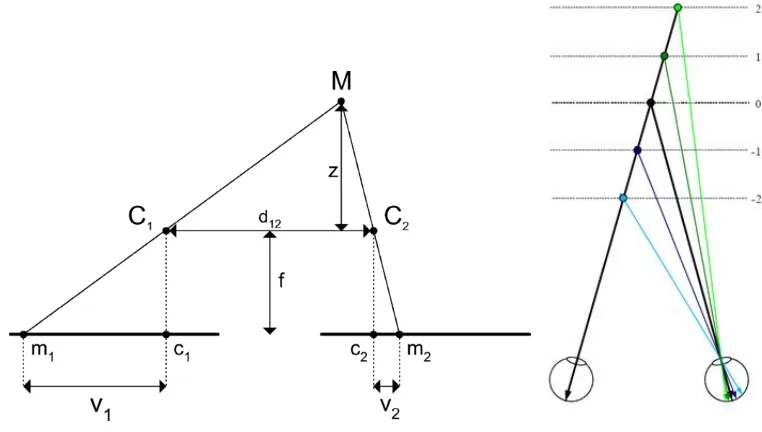
Like the human visual system, you can place two cameras at a certain distance from each other and receive an image from two slightly different points view.
In humans, these distinct images are used to estimate the depth and fuse together to create a single image of the scene.
The estimation of disparities is the problem of finding corresponding points in a pair of stereo images to calculate the distance of the object. Il literature are large number of stereo algorithms are presented, but only a few are tailored for custom sensors [45][46]. In fact, most of the activity on image processing, developed by the scientific community, has been based and tailored on standard imagers. It s therefore difficult to share and to exploit this know-how on a custom sensor architecture.
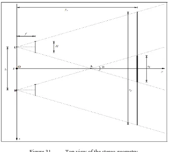
plane, a model based on an ideal optical camera is used. This model does not include any distortion due to the lenses. Moreover, the image plane is considered to be continuous, while many current sensors, being composed of cells, have, in fact, only quantized coordinates. Given the simplifications assumed, it is considered an ideal model of camera; it is representative and useful because it allows us to focus on complex geometry, avoiding the complications due to the complex optical geometry of the real objectives and inevitable spurious factors, including distortions and aberrations, which occur in practice. Imagine placing two cameras on the same x axis (symmetrical points in respect to y axis) positioned in the same direction parallel to y and lying on the z = 0 Figure 31.
Figure 31. Top view of the stereo geometry.
This baseline can effect on their respective image plane named disparity. It’s possible to understand the object distance trough the disparity exploitation.
Figure 32. Top vision from the pattern of cameras and differente disparity proiection.
Now the stereo probleme it’s a correspondence problem, can be solved using an algorithm that scans both the left and right images for matching image features.
In literature several algorithms exist and they can be divided in two groups: - Correlation based
- Feature based
In the Correlation based algorithm it’s possible adopt local or global methods, the disparity is evaluated using a winner-take-all (WTA) strategy.
calculating: Normalized Cross Correlation (NCC), Sum of Squared Difference (SSD) or Sum of Absolute Difference (SAD).
Normalized correlation:
2 2 ) , ( ) , ( ) , ( ) , ( y x R y x L y x R y x L Sum of squared differences:
L(x,y)R(x,yd)
2 Sum of absolute differences:
L(x,y)R(x,yd)
Moreover, the windows size is a trade-off because in a small area images are more similar despite of different view points, but in big areas, the ratio of signal to noise increases. These algorithms are suitable to treat a wide variety of images and provide a dense depth maps.
The feature-based algorithms face the problem of correspondence at a higher level than correlation-based. The first step is to identify items or groups of points in the stereo pair with certain features: edges, lines or angles. The differences between feature-based and correlation-based algorithms consist in the fact that the first exploit additional information in order to apply the matching, for instance the orientation or length of the edges. This is the main limit, because it is not always possible to know the type of feature a before as it depends on the applications.
Our kind of images does not allow the use of classical philosophy to calculate the disparity because our sensor does not provide conventional images as seen above. For these reason is necessary to develop a new custom algorithm able to exploit the peculiarity of sensor efficiently.
Figure 33. Sensor image date deliver in spars matrices organization.
This sensor execute a pre elaboration of the image extracting the edge present in the scene directly on chip and deliver a spar matrices organized in this way. In this scene are presented 13 pixels and only the corresponds address are delivered in a raster scan order. Figure 33.
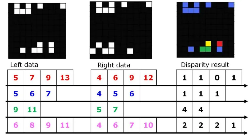
Figure 34. The pair of images left and right respectively e the ideal result the disparity algorithm
Figure 34. Figure 35. describes the problem to be resolved, in the top part is possible to see the left and right images delivered by the sensors, on the right there is the image we wont to obtain by algorithm.
In this last image every pixel is coded with the a color which represent the depth of that pixel.
Below the previous images the corresponding data coding is shown.
The task is to takes advantage from the characteristics of the sensor evaluate the disparity of object present in each scene, starting on this positional data coding.
Figure 35. In vertical line we represented a row of left image end in horizontal we represented the
In order to explain the objective of this algorithm we represent the possible matches in Figure 35. , where in vertical line we have represented a row of left image end in horizontal we have represented the same row delivered by the right sensor.
Looking at this representation is necessary to define some constraints: - Epipolar (The disparity is evaluated only row by row)
- Uniqueness (It’s possible to find only one correct match between left end right rows)
- Ordered (The sensor deliver the address in ascending order)
- Disparity limit (Knowing the geometry of the system is possibility to limit the maximum disparity evaluated).
Bleak point represents the active pixel in the same row, red represents the possible candidate matching and in green the correct match. And the diagonal line represent the same disparity information for any mach associated.
The idea looking at the data is to adopt the Graph Theory [47][48][49]. This type of approach is a mathematical structures used to model pair wise relations between objects from a certain collection, in this case the addresses of the pixels from left and right imager.
In the theory graph the interconnected objects are represented by mathematical abstractions called vertices(green), and the links that connect some pairs of vertices are called edges(blu).see in Figure 36.
Figure 36. Two corrispondent row and the disparity.
The goal of the function cost is to balance the point skipped and the disparity related associating the minor cost to correct match Dijkstra inspired [58].
In order to do this, the function cost is to builder including three principal element, the first and second element evaluate the point skipped in left and right scanline. In other word the non adjacent address value are penalized and the last term the variation of disparity respect the last match found, normalized with the distance between the adjacent pixels.
We consider this correct sequence matching:
i
kli
qr
i
jli
pr
S
j,p
,,
,...
,,
, for k,j,p,q∈{1,2,…,M} (1)The function cost associated is:
I II III
j p jp
M r p r p l j l j p j p
j A i i i i f d d
S
C 1, 1 ,
1 1 , 1 , , 1 , ,
, 1 1 ,
(2)The idea is to build a cost function C(S) computed for any possible match between the corresponding rows of left and right imagers. In this way the stereo correspondence problem turns into a cost function minimization problem.
A represents the balancing coefficient which is used to calculate the cost function contribute of the new pixel added to a sequence, typically set to 0.5 (this parameter is connect to the distribution of the pixels). The last term on the rights the change in disparity, normalized with respect to the distance between the pixels in the left row, which can be expressed as:
l j l j l p l j l p l j p j lj i i
i i i i i i p j j p j p j l l r l r l l l d d d d f , 1 , , 1 , 1 , , 1 , 1 , 1 , 1 , 1 , 1 ,
(3)
In this case for any pare of two pixels delivered by the left and right sensors a function cost will be defined.
The cost function C(s) is additive. For a given Sj,p ending in (ij,l, ip,r), the cost function C(Sj+1,p+1) of the next sequence, adding the term (ij+1,l,ip+1,r), is obtained by simply adding the term:
ij1,l ij,l 1 ip1,r ip,r 1
f dj,p,dj1,p1
A (4)
to the previous C(Sj,p).
Here, the next matching is not necessary referred to the next pixel located in the memory, but has to be found elsewhere inside the row.
Eq.(5) it is solved through dynamic programming; for any j and p pair, addressing the pixels in the memory, the cost function is computed with respect to all the pixels placed in the memory. Eq.(5) has a complexity M4, where M is the number of pixels in the row of the sensor. This is a worst case estimation, due to four nested embedded loops connected to j, p, v, w parameter. However, under some assumptions the complexity of the problem can be significantly reduced without affecting the overall algorithm reliability. Rather than involving all the pixels of the row in the matching computation, only those located in the neighborhood can be involved by limiting the values of v and w in eq.(5).
Figure 37. Example of cost function constraint.
Figure 37. shows an example of cost function calculation under the following assumptions:
- matching pixel neighborhood v, w = 3
- maximum admitted disparity is dj=6 pixel. (this value depends on the specific geometry of the optical system);
4.2.
Stereo vision system simulation
After the implementation algorithm it’s necessary to validate the results applying the algorithm on a image characterized by the conventional resolution adopted for people monitoring. In order to quantitatively evaluate a disparity estimation approach develop a standard data-set with disparities is required.
First to test the stereo algorithm develop is necessary to simulate the data delivered by the sensor algorithm on stereo pedestrian data-set. Unfortunately, standard disparity data-sets, such as the Tsukuba, Venus, or Map data-sets may not be applicable for people monitoring algorithms. In fact these dataset include some ambiguous periodical pattern difficult discriminated only by binary edge detection. It’s necessary to adopt a data set rectified and synchronized (Overhead Scenario 2D pedestrian detection
http://www.cdvp.dcu.ie/datasets/pedestrian_detection/).
a) b)
c) d)
Figure 38. Simulationa results a)Left binary image b)Right binary image c)Real scene
d)Disparity resoults.
4.3.
System specifications an realization
Figure 39. Top vision from the pattern of cameras.
The main element are: System coordinates;
- x y z : coordinate word;
- xSL ySL : coordinate left sensor; - xRL yRL : coordinate right sensor; System coordinates
- f : focal length;
- H : horizontal size of the sensors;
- NH: horizontal resolution (number of pixels); - NR: horizontal size of a pixel ;
- b : baseline represent distance between sensors. Other sizes
- P : point in the real world coordinate (xp, yp, 0); - H : horizontal size of the sensors;
H R
N H
The PL coordinates are (XpSL, 0) while those of PR are (XpSR, 0). The visible area from both cameras is bounded by:
H fb OA f H arcan 2 2
(6)
Figure 40. Top vision from the pattern of cameras.
With reference to Figure 40. Figure 39. we consider a parallel plan to XZ positioned with a distance Yr from the origin. The two cameras don’t see the same part of that plan; if yr OAintersection between two images is null. In the bi-dimensional scheme
the plan is represented by a straight line and the intersection of two visions by a segment of a length of:
f fb Hy r r S
(7)
The union is instead represented by a segment of a length of:
f fb Hy r r T
(8)
fb Hy fb Hy r r r r r T S
(9)
The degree of overlapping does not depend only on the parameters of the system, but also on the distance yr. Assuming that the algorithm for stereo analysis has particular requirements r>rrmin we have an estimate on the minimum distance:
H fb r r yr min min 1 1 (10) These equations can be used to select the cameras more appropriate for a certain application. The angle α, the distance minimum and the maximum of the objects can be estimated from parameters of the cameras and the appropriate assumptions
t : minimum measurable disparity from stereo algorithms;
n : size of the more discoverable small object measured in pixels; Δx : size of small object that you want to detect;
a : ratio of maximum permissible uncertainty on the distance of an object and its actual distance;
Rmin : minimum degree of overlapping for stereo analysis.
R R nH x f tH fb a a y , 1 min
min (11)
H fb r r H fb r r H fb y min min min min max 1 1 1 1 , max (12)
After these mathematical considerations it is necessary to set the constraints for a particular application and to adopt a stereo algorithm for obtaining disparity maps. For our people counting applications we position the system at a height of 3m and see 1 to 2 meters away.
We fix: t = 1, a = 0,25 % , r = 85% , b = 8 Cm.
Figure 41. Laboratory Stereo vision simulation.
Figure 42. This picture represents left and right vision extracted by the same camera.
Figure 42. shows the setup realized in the laboratory to simulate the stereo visions. Only one sensor was mounted on a triple axes rail, allowing it to be shifted along the axes: Y (lateral), Z (depth). By using this system, the following results have been obtained:
Real distance (DR): DR=0,6m (with 6mm optics),
Estimated distance (D): disparity 28 pixel(shoulders), distance 0,65m, error 0,05 ≈ 8% As we can see in the image there is a difference between the two shots of about 28 pixels.
Through geometric calculations, are able to calculate the distance from the system:
r
H d
f b D
This error is caused by the low resolution of the sensor, using two cameras this error will be larger because it introduces new parameters that characterize the diversity of the two sensors as different focal lengths, misalignment, etc., these problems are solvable with the calibration.
To realize the first prototype tests, a board was designed through the Orcad software exploitation. The aim of the board is to create, starting from two sensor a single device easily connectable with a single FPGA. The second sensors were placed on the board at a distance regulated by the epipolar geometry, in particular controlled by the formulas (11) (12) illustrated above, fixing some parameters related a type of approximately 1.5m wide and 3m fixing in height.
The baseline was fixed at 8 cm, using a varifocal lens from 2.9 to 8.2mm, whit a zoom that could adapt the geometry for different situation. On the board mounted point where installed to allow the alignment of the sensors with the optics.
Figure 43. First Stereo prototype
The FPGA, Xilinx Spartan-3 has been selected for the development phase. In particular, XEM3001 Module [51], has be used, offering sufficient flexibility and complexity for the specific application.