An investigation of the Ora del Garda wind by means of airborne and surface measurements

(1)

Doctoral School in Environmental Engineering

An investigation of the

Ora del Garda

wind

by means of airborne and surface

measurements

Lavinia Laiti

(2)

Doctoral thesis in Environmental Engineering, XXV cycle

Department of Civil, Environmental and Mechanical Engineering, University of Trento Academic year 2011/2012

Supervisor: Dino Zardi, University of Trento

On the cover: view of the northern shoreline of Lake Garda from the panoramic trail between Busatte and Tempesta.

This thesis is partially based on:

Laiti, L., Zardi, D., de Franceschi, M., Rampanelli, G., 2013. Residual kriging analysis of airborne measurements: application to the mapping of atmospheric boundary-layer thermal structures in a mountain valley. Atmos. Sci. Lett. 14, 79-85.

Laiti, L., Zardi, D., de Franceschi, M., Rampanelli, G., 2013. Atmospheric boundary-layer structures associated with the Ora del Garda wind in the Alps as revealed from airborne and surface measurements. [submitted to Atmos. Res.]

University of Trento Trento, Italy

(3)

(4)

(5)

Aknowledgements

I would like to thank my supervisor, prof. Dino Zardi, for his support during these years. Thanks also to Dr. Massimiliano de Franceschi for the fruitful discussions, and for providing the data of the field campaign of summer 2001.

Thanks to the Trento University Sport Center (CUS Trento) for providing the motorglider, and to the pilot Fabrizio Interlandi for performing the flights.

(6)

(7)

Contents

List of Figures . . . V

List of Tables . . . XV

Summary . . . 1

Chapter 1 Introduction . . . 3

1.1 Introduction . . . 5

1.2 Motivation and rationale of the thesis. . . 6

1.3 Thesis outline. . . 8

Chapter 2 The Ora del Garda wind . . . 11

Abstract . . . 11

2.2 Description of the study area. . . 17

2.3 The Ora del Garda development. . . 20

2.4 An example of typical Ora del Garda diurnal cycle. . . 21

2.5 Summary. . . 27

Chapter 3 Outline of airborne and surface measurements. . . 29

Abstract . . . 29

3.2 The airborne measurement platform. . . 32

3.3 General outline of airborne measurements . . . 33

3.4 24 September 1998 flight (flight #1) . . . 34

3.4.1 Description of the flight. . . 34

3.4.2 Weather conditions and surface observations . . . 35

3.5 05 August and 01 September 1999 flights (flights #2 and #3) . . . 39

3.5.1 Description of the flights. . . 39

3.5.2 Weather conditions and surface observations . . . 39

3.6 23 August 2001 flights (flights #4 and #5) . . . 44

3.6.2 Weather conditions . . . 46

(8)

3.6.3.1 a) Lower Sarca Valley. . . 48

3.6.3.2 b) Lakes Valley . . . 51

3.6.3.3 c) Adige Valley south of Trento. . . 52

3.6.3.4 d) Adige Valley north of Trento. . . 52

3.7 Summary. . . 54

Chapter 4 Methods for the post-processing of airborne data. . . 57

Abstract . . . 57

4.2 The test-bed dataset . . . 60

4.2.1 Description of the target area. . . 60

4.3 Correction of the sensor time-lag effect. . . 62

4.3.1 Theoretical framework. . . 62

4.3.2 Determination of the effective sensor time constant. . . 66

4.4 The interpolation methods. . . 70

4.4.1 Inverse distance methods. . . 70

4.4.2 Natural neighbor method. . . 71

4.4.3 Residual kriging method. . . 72

4.4.3.1 The pseudo-soundings . . . 72

4.4.3.2 The semivariogram function . . . 75

4.5 Comparison of the methods. . . 77

4.5.1 Cross-validation analysis . . . 77

4.5.2 Critical comparison of the interpolated fields. . . 82

4.6 Evolution of the ABL thermal structure. . . 88

4.7 Summary . . . 90

Chapter 5 Deciphering the dominant vertical structure of the valley atmospheric boundary-layer . . . 93

Abstract . . . 93

5.2 24 September 1998 (flight #1) . . . 97

5.3 05 August and 01 September 1999 (flights #2 and #3) . . . 100

5.3.1 General features of the valley ABL. . . 100

5.3.2 Local features of the valley ABL. . . 104

5.4 23 August 2001 (flights #4 and #5) . . . 104

5.4.1 ABL structure in the lower Sarca Valley and Lakes Valley. . . 107

(9)

5.5 Summary. . . 110

Chapter 6 Deciphering the fine-scale structure of the valley atmospheric boundary-layer. . . 113

Abstract. . . 113

6.2 24 September 1998 (flight #1) . . . 117

6.3 05 August and 01 September 1999 (flights #2 and #3). . . 121

6.3.1 Lower Sarca Valley - Lake Garda shoreline area. . . 121

6.3.2 Lakes Valley - Cavedine Lake area . . . 123

6.3.3 Lakes Valley - Terlago saddle area. . . 125

6.3.4 Adige Valley - interaction area . . . 127

6.4 23 August 2001 (flights #4 and #5) . . . 130

6.4.1 Lower Sarca Valley. . . 130

6.4.2 Lakes Valley. . . 133

6.4.3 Interaction area. . . 134

6.5 Summary. . . 137

Chapter 7 . . . 141

Conclusions and future developments . . . 141

7.1 Conclusions. . . 143

7.2 Outlook on future developments. . . 145

(10)

(11)

List of Figures

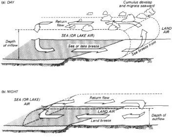
Figure 2.1. Schematic diagram of a) sea and b) land breeze circulations developing across a shoreline by day and night respectively, during fair-weather conditions. Notice the leading edge of the sea breeze, i.e. the sea-breeze front, formed by colder and more humid marine air moving onshore and wedging under the warmer land air (from Oke 1987). . . 13

Figure 2.2. Defant’s (1949) scheme of diurnal slope and valley wind regimes. From the top:

A) at sunrise the down-valley wind still blows while up-slope winds start to develop, B)

in the morning transition phase up-slope winds are fully developed, C) at noon up-slope winds weaken and the up-valley wind starts to blow, D) in the late afternoon the up-valley wind is fully developed, E) at sunset the up-valley wind weakens and down-slope winds start to develop, F) in the late-evening transition phase down-slope winds are fully developed, G) in the first hours of the night down-slope winds weaken and the down-valley wind develops, H) before sunrise down-slope winds cease and the down-valley wind is fully developed. . . 15

Figure 2.3. a) Localization of the target area (indicated by the rectangular box) near Trento city and Lake Garda, in the southeastern Italian Alps. b) Topography of the study area (contour interval: 200 m); the dashed arrow marks the path followed by the Ora del Garda wind along the lower Sarca Valley and Lakes Valley, from the northern shoreline of Lake Garda to the saddle of Terlago, and finally to the Adige Valley north of Trento. Cavedine and Toblino lakes are also indicated, as well as some reference towns in the area (Trento, Riva del Garda, Arco and Terlago). Coordinate system: Gauss Boaga, Italy East fuse. . . . 18

Figure 2.4. 3D view of the topography of the the lower Sarca Valley facing the northern shoreline of Lake Garda (view is from S). Mt. Brione relief is indicated. The white arrow marks the corridor communicating the lower Sarca Valley with the Lakes Valley farther north. Image © Google Earth, © 2013 GeoEye. . . 18

(12)

Figure 2.6. Altimetric profile of the floor of the valleys where the Ora del Garda wind blows (dark grey shading), from the northern shoreline of Lake Garda (black shading) to the Terlago saddle, where the wind finally breaks out into the underlying Adige Valley (the wind path is indicated by the dashed arrow). The profiles of the lateral crests are shown for both the valley sides, and the most important topographic features of the area are also reported. . . . 20

Figure 2.7. Localization of the AWSs considered in the climatologic analysis performed for the 18-21 August 2012 period, from Lake Garda shoreline to the Terlago saddle ridge, and the Adige Valley (view is from SE). Image © Google Earth, © 2013 Cnes/Spot Image, © 2013 DigitalGlobe, © 2013 European Space Imaging, © 2013 GeoEye. . . 22

Figure 2.8. Daily cycles of solar radiation at the AWSs considered in the climatologic analysis performed for the 18-21 August 2012 (see figure 2.7 for locations). Notice that all the cycles present a very regular pattern, (except at PIE, where the shadowing by some obstacle, possibly a tree, causes a morning radiation deficit occurring everyday), indicating very clear-sky conditions for the selected days. . . 24

Figure 2.9. Daily cycles of wind speed and direction as time series of wind vectors at the AWSs considered in the climatologic analysis performed for the 18-21 August 2012 (see

figure 2.7 for locations and table 2.1 for anemometer heights). Notice that the wind vectors have been projected onto the local valley axis direction (22.5° N for RDG, ARC, DRO, PIE; 45.0° N for SAR; 67.5° N for TER; -22.5° N for GAR; 0.0° N for TNS), so that in this representation vertical and horizontal components represent respectively along-valley and cross-valley wind components. The sequence is from the AWS closest to Lake Garda shoreline (RDG), at the bottom of the graph, to the farthest (TNS), at the top. Accordingly the Ora del Garda wind development can be followed along the Sarca and Lakes Valley until the Adige Valley, reading the graph from the bottom to the top. . . . 25

Figure 2.10. Daily cycles of down-stream wind speed (i.e. the wind component locally associated to the Ora del Garda and Adige Valley wind flow) at the AWSs considered in the climatologic analysis performed for the 18-21 August 2012 (see figure 2.7 for locations and table 2.1 for anemometer heights). The local orientation adopted for the valley axis is reported in figure 2.9 caption. (*) Notice that for GAR the cross-valley component is displayed as down-stream component, instead of the along-valley component shown for all the other AWSs. . . 26

(13)

Figure 3.1. The Scheibe Falck SF 25C. Notice temperature and humidity sensors mounted on the left-side leg of the motorglider undercarriage (lower-right corner of the picture).

Picture by courtesy of Massimiliano de Franceschi. . . 32

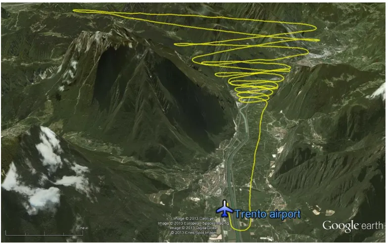
Figure 3.2. 3D representation of flight #1 trajectory (yellow line). View is from S. The name of the vertical sections explored by each single spiral are also indicated (labelled according to the site they explored). Image © Google Earth, © 2013 European Space Imaging, © 2013 GeoEye, © 2013 Cnes/Spot Image, © 2013 DigitalGlobe. . . 35

Figure 3.3. Location of RDG, ARC1, TNS and PAG surface weather stations in the study area. View is from SE. Image © Google Earth, © 2013 DigitalGlobe, © 2013 Cnes/Spot Image, © 2013 GeoEye, © 2013 European Space Imaging. . . 36

Figure 3.4. Time series of wind (vectors) observations at RDG, ARC1 and TNS surface stations for 24 Sep 1998. Flight #1 duration is indicated by the grey band. N direction is top, S is bottom, W is left, E is right. . . 37

Figure 3.5. Time series of radiation (grey shading), temperature (solid black line) and water vapour mixing ratio (dashed black line) observations at RDG, ARC1 and TNS surface stations for 24 Sep 1998. Flight #1 takeoff and landing times are indicated by vertical lines. . . 38

Figure 3.8. As in figure 3.4, but for flight #2. . . 41

(14)

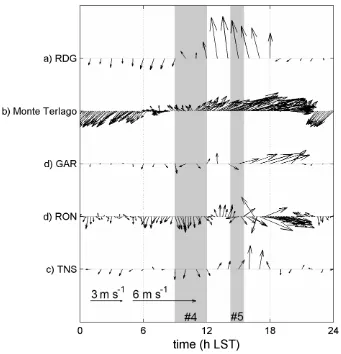
Figure 3.15. Time series of wind observations (vectors) at RDG, Monte Terlago, GAR, RON and TNS surface stations for 23 Aug 2001. The duration of flights #4 and #5 is indicated by the grey bands. The spatial development of the Ora del Garda wind along the lower Sarca Valley (a), the Lakes Valley (b) and finally the Adige Valley, both north (d) and south of Trento city (c), can be read from the top to the bottom of the graph. N direction is top, S is bottom, W is left, E is right. . . 49

Figure 3.16. Time series of 2 m AGL temperature observations at selected surface stations (listed in table 3.6) for 23 Aug 2001. RDGw time series represents water temperature observations at RDG station. The duration of flights #4 and #5 is indicated by the grey bands. The stations are grouped according to their geographic area (see table 3.6). . . . 50

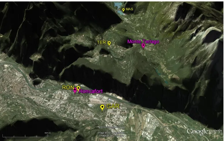
Figure 3.17. Location of the surface stations considered in the analysis of the Ora del Garda

cycle on 23 Aug 2001 in the flat basin facing Lake Garda shore. Station labels refer to

Figure 3.18. Location of the surface stations considered in the analysis of the Ora del Garda

Figure 3.19. Time series of SHF from eddy covariance analysis (averaging interval: 30 min) of ultrasonic anemometer observations at Roncafort site (see figure 3.18) for 23 Aug 2001. . . . 54

Figure 4.1. 3D representation of flight #N trajectory exploring the target Adige Valley cross section. View is from N. Image © Google Earth, © 2013 GeoEye, © 2013 European Space Imaging, © 2013 DigitalGlobe, © 2013 Cnes/Spot Image.. . . 61

Figure 4.2. Original observations of temperature (left) and potential temperature (right) provided by the RTD sensor for flights #M (black), #N (red) and #A (blue). Solid lines indicate the flight ascents, while dashed lines represent the flight descents. . . 63

Figure 4.3. Vertical profiles of true (black line) and measured (grey line) air temperature (left) and potential temperature (right), resulting from the conceptual experiment by Rampanelli (2004), for a steady-state CBL condition. Ascents are solid lines, while descents are represented by dashed lines. Simulation parameters are: T0 (temperature at

the ground surface) = m = 288 K, h = 700 m, H (maximum flight height) = 2300 m, wa

(climbing vertical speed) = 1.5 m s-1, wd (diving vertical speed) = 2.5 m s-1,  = 35

s.. . . 63

(15)

temperature value detected in the lowest layers: the combination of the slow sensor response and the gradual heating of the ML with time reduces the hysteresis loop amplitude inside the lowest ABL. . . 44

Figure 4.5. Close-up on the measured temperature hysteresis loop at the top of the ideal flight trajectory (conceptual experiment results). The black line is the true atmospheric temperature Ta(t), while the black line is the temperature indicated by the instrument T(t). Ascending and descending branch of the flight are respectively solid lines and dashed lines. The total loop amplitude ΔT is also indicated.. . . 67

Figure 4.6. Observations of temperature (left) and potential temperature (right) after the correction of the RTD sensor time-lag effect for flights #M (black), #N (red) and #A (blue). Solid lines indicate the flight ascents, while dashed lines represent the flight descents. Notice in particular the fact that the hysteresis loops present in figure 4.2 in the uppermost part of the profiles (i.e. FA) have been removed by the application of the deconvolution algorithm. On the contrary, the evolution of the ABL (i.e. the heating of the lowest atmosphere) during the single flight time has become evident (except for flight #A).. . . 68

Figure 4.7. Upper panel: longitude time series for the ascending branch of flight #M (in km E; geographic coordinate system: Gauss Boaga, Italy East fuse). Lower panel: corresponding time series of original measured RTD temperature (grey line), RTD temperature corrected for the slow-response effect (solid black line) and temperature recorded by the thermohygrometer (dashed black line). The arrows highlight the good correspondence between local temperature peaks and the turning points of the flight trajectory, where the motorglider flew close to the western valley sidewall. The backward time shift (approximately equal to ) produced by the application of the deconvolution algorithm can also be appreciated. . . 69

Figure 4.8. Vertical distribution of potential temperature observations for the three flights #M, #N and #A. The superimposed solid lines are the pseudo-sounding extracted from these data, and adopted as drift terms in RK for the evaluation of residuals (colors correspond to those used in figures 4.2 and 4.6). The arrows indicate the top of the detected MLs. The grey shading marks the local valley-floor height (180 m MSL), while the black horizontal lines report the local height of the lateral crests, respectively on the western (solid line) and on the eastern side (dashed line) of the valley.. . . 73

(16)

close to it. . . 74

Figure 4.10. Horizontal (i.e. cross-valley) (x), vertical (z) and omnidirectional (omni)

empirical semivariograms of potential temperature residuals for flight #A (markers). Associated lines represent the best-fit theoretical semivariograms (spherical model for x,

exponential model for z and omni). Practical range values for the directional

semivariograms are respectively 2230 m in cross-valley direction and 580 m in vertical direction, thus determining an anisotropy ratio of 3.8, which is used to isotropize the field before computing omni (practical range: 650 m). . . 76

Figure 4.11. LOOCV results for flight #M: scatterplots of observed vs. predicted values of potential temperature for each interpolation method. R-IDW, R-exp-ISD and R-NN refer to the adoption of a residual approach for IDW, exp-ISD and NN methods respectively. The black lines represent identity between observed and predicted values. . . . 79

Figure 4.12. As in figure 4.11 but for flight #N. . . 80

Figure 4.13. As in figure 4.11 but for flight #A. . . 81

Figure 4.14. Interpolated potential temperature field (in K) from flight #M for all the interpolation methods compared. Contour interval is 0.5 K (in white). The black dashed line represents the projection of the trajectory followed by the motorglider. The local valley section topography is indicated in grey shading. . . 84

Figure 4.15. As in figure 4.14, but for flight #N. . . 85

Figure 4.16. As in figure 4.14, but for flight #A. . . 86

Figure 4.17. RK-estimated standard deviation of the interpolated potential temperature field for the three flights (in color). Contour interval is 0.1 K (in white). The black dashed line represents the projection of the trajectory followed by the motorglider onto the median vertical planes of the interpolation grids. The local valley section topography is indicated in grey shading. . . . 87

Figure 4.18. RK-interpolated potential temperature field from flight #M. Contour interval is 0.5 K (in white). The black dashed line represents the projection of the trajectory followed by the motorglider. The local valley section topography is indicated in grey shading. . . 89

Figure 4.19. As in figure 4.18, but for flight #N. . . 90

Figure 4.20. As in figure 4.18, but for flight #A. . . 90

(17)

in the deep ML, extending from above the unstable surface layer to the basis of the strongly-stable inversion layer capping the ABL (modified from Kaimal and Finnigan 1994).. . . 95

Figure 5.2. Potential temperature measurements (black dots) at each valley cross section for flight #1 compared to routine surface observations from nearby stations (grey bullets; see section 3.4.2 and 3.6.3 for station labels and positions). Grey lines are the pseudo-soundings representative of the mean vertical structure, and used as drift terms for the evaluation of residuals in the residual kriging procedure (labeled as in table 5.1). Magenta and blue lines represent 1200 UTC (i.e. 1300 LST) soundings from LIML and LIPD stations respectively (see figure 5.3). The local valley-floor height for each cross section is indicated by the grey shading.. . . 98

Figure 5.3. Location of the stations (yellow placemarks) providing routine soundings for the comparison with the pseudo-soundings extracted from the airborne data. LIML is Milano-Linate airport, LIPD is Udine-Campoformido airport, LOWI is Innsbruck-Kranebitten airport. The study area is delimited by the rectangular box. Image © Google Earth, © Geoimage Austria, © 2013 TerraMetrics, © 2013 Cnes/Spot Image, © 2013 GeoContent. . . 99

Figure 5.4. Observed pseudo-soundings of potential temperature, compared to routine soundings and surface observations for flight #2 and #3. Black and grey lines are airborne pseudo-soundings for each single explored valley section, labeled as in table 5.2. Color lines are associated with symbols indicating observations from the surface stations nearest to the respective spirals (see section 3.4.2 and 3.6.3 for station labels and positions); RDG, CAV and MAS stations are located on a lake shore. Thinner lines are 1200 UTC (i.e. 1300 LST) soundings from LIML, LIPD and LOWI stations (see figure 5.2). . . . 101

Figure 5.5. As in figure 5.4, but for water vapour mixing ratio. . . 102

Figure 5.6. Observed pseudo-soundings of potential temperature, compared to routine soundings and surface observations for flight #4 and #5: a) lower Sarca Valley and Lakes Valley (flight #4) b) upper Lakes Valley and Adige Valley (i.e. interaction area; flights #4 and #5). Black and grey lines are airborne pseudo-soundings for each single explored valley section, labeled as in table 5.3. Lines are associated with symbols indicating observations from the surface stations nearest to the respective spirals (see section 3.6.3

for station labels and positions). Color lines are 0600, 1200 and 1800 UTC (i.e. 0700, 1300 and 1900 LST) soundings from LIML and LIPD stations (see figure 5.3) . . . 105

(18)

Figure 6.1. 3D representation of flight #1 trajectory (yellow line). The vertical planes adopted for displaying the RK-interpolated potential temperature fields in figure 6.2 are also indicated. Image © Google Earth, © 2013 Cnes/Spot Image, © 2013 European Space Imaging, © 2013 GeoEye, © 2013 DigitalGlobe. . . 117

Figure 6.2. RK-interpolated potential temperature field for a) spiral A-1. Contour interval is 0.25 K (in white). The black dashed line represents the motorglider trajectory. The valley section topography is indicated in grey shading. b) As in panel a), but for spirals B/w-1 (left) and B/e-1 (right). The black arrow indicates Cavedine Lake’s position at the valley bottom. c) As in panel a), but for spiral C-1. . . 119

Figure 6.3. RK-interpolated anomalies of potential temperature (i.e. deviations from pseudo-sounding values) on horizontal planes at various vertical levels for spiral C-1 (figure 6.2c). The upper panel shows the profile of the underlying topography on a vertical cross section. The latter intersects each horizontal plane at the dotted line labelled with the corresponding letter. White areas denote regions where the topography elevation exceeds the height of the horizontal plane, or regions outside the maximum acceptable interpolation distance. The black curve is the projection of the flight trajectory on the planes. The abscise axis is the same as in figure 6.2c. . . 120

Figure 6.4. 3D representation of flight #2 (yellow line) and #3 (red line) trajectories. The vertical planes adopted for displaying the RK-interpolated potential temperature fields in figures 6.5-6.11 are also indicated. Image © Google Earth, © 2013 Cnes/Spot Image, © 2013 European Space Imaging, © 2013 GeoEye, © 2013 DigitalGlobe. . . 121

Figure 6.5. Vertical section of RK-interpolated potential temperature field for spiral A-2 from flight #2 (see corresponding vertical plane in figure 6.4); contour interval is 0.25 K (in white). The black dashed line indicates the trajectory followed by the motorglider over the considered section. The correspondent valley topography is indicated in light grey (Mount Brione profile is also reported), while dark grey indicates Lake Garda. The black triangle shows Lake Garda shoreline (accordingly, the horizontal coordinate can be read as distance from shoreline in SSW-NNE direction). . . 122

Figure 6.6. As in figure 6.5, but for spiral A-3 from flight #3. . . 123

Figure 6.7. As in figure 6.5, but for spiral B-2 from flight #2 (B-2 plane in figure 6.4). The black arrow shows the position of Cavedine Lake. Horizontal coordinate marks the cross-valley direction (Lakes Valley; WNW-ESE direction). . . . 124

Figure 6.8. As in figure 6.5, but for spiral B-3 from flight #3 (B-3 plane in figure 6.4). The black arrow shows the position of Cavedine Lake. Horizontal coordinate marks the cross-valley direction (Lakes Valley; WNW-ESE direction). . . . 125

(19)

Horizontal coordinate marks the cross-valley direction (Lakes Valley; WNW-ESE direction). Note that the intermediate levels (between 800 and 1500 m MSL) of the northwestern half (i.e. left) of the valley cross section were not entirely explored by the flight; as a consequence, potential temperature values in this region result from an extrapolation process and thus present poor reliability. . . 126

Figure 6.10. As in figure 6.5, but for spiral C-3 from flight #3 (C-3 plane in figure 6.4). Horizontal coordinate marks the cross-valley direction (Lakes Valley; WNW-ESE direction). . . . 127

Figure 6.11. As in figure 6.5, but for spiral D-3 from flight #3 (D-3 plane in figure 6.4). The black arrow shows the point from where of the Ora del Garda wind overflows from the Lakes Valley, i.e. the saddle of Terlago. Horizontal coordinate marks the cross-valley direction (Adige Valley; W-E direction). . . 128

Figure 6.12. RK-interpolated potential temperature anomaly (in colors) at different height levels (indicated in figure 6.11) for section D-3 from flight #3. The upper panel shows the underlying Adige Valley topography: contour interval is 100 m, the valley floor (~200 m MSL) is colored in grey; the valley sidewall on the left is the saddle of Terlago. The black line is the horizontal projection of the motorglider trajectory. Abscise coordinates correspond to cross-valley coordinates in figure 6.11 (W-E direction) . . . . 129

Figure 6.13. 3D representation of flight #4 (yellow line) and #5 (red line) trajectories. The vertical planes adopted for displaying the RK-interpolated potential temperature fields in figures 6.14-6.18 are also indicated. Image © Google Earth, © 2013 Cnes/Spot Image, © 2013 European Space Imaging, © 2013 GeoEye, © 2013 DigitalGlobe. . . 130

Figure 6.14. Transversal (i.e. cross-valley) vertical section of RK-interpolated potential temperature field for spiral A-4 from flight #4 (see corresponding vertical plane A/c-4 in

figure 6.13); contour interval is 0.25 K (in white). The correspondent valley topography is indicated in grey. The cross section is taken immediately down-stream of the Monte Brione relief (semi-transparent shading), i.e. 3 km inland from the Lake Garda shoreline. Accordingly, the horizontal coordinate marks the cross-valley direction (lower Sarca Valley; WNW-ESE direction). The black dashed line indicates the trajectory followed by the motorglider over the considered section. . . 132

Figure 6.15. Longitudinal (i.e. along-valley) vertical section of RK-interpolated potential temperature field for spiral A-4 from flight #4 (see corresponding vertical plane A/l-4 in

(20)

middle of the lower Sarca Valley. The black dashed line indicates the trajectory followed by the motorglider over the considered section. The black triangle shows Lake Garda shoreline. Accordingly, the horizontal coordinate marks the along-valley direction (lower Sarca Valley; SSW-NNE direction). . . 133

Figure 6.16. As in figure 6.14 but for spiral B1-4 from flight #4 (see corresponding vertical plane B1-4 in figure 6.13). Accordingly, the horizontal coordinate marks the cross-valley direction (WSW-ENE direction). . . 134

Figure 6.17. As in figure 6.14 but for spiral C-5 from flight #5 (see corresponding vertical plane C-5 in figure 6.13). Accordingly, the horizontal coordinate marks the cross-valley direction (upper Lakes Valley; N-S direction). . . 135

(21)

List of Tables

Table 2.1. List of the AWSs considered in the climatologic analysis performed for the 18-21 August 2012 period. AWS names refer to the ones indicated in figure 2.7. Each AWS elevation is also reported, together with the height of the installed anemometer. All the stations are operated by Istituto Agrario di S. Michele all’Adige - Edmund Mach Foundation. . . 23

Table 3.1. List of the meteorological sensors carried by the motorglider and main technical specifications. . . 33

Table 3.2. Timings and characteristics of measurement flight #1. Single spirals are labelled according to figure 3.2. CV and AV respectively indicate whether the spiraling trajectories explored a cross- or an along-valley oriented section. D stands for a descending (downward) flight leg and U for an ascending (upward) flight leg. LST times are UTC+1 times. . . 35

Table 3.3. List of surface weather stations considered in the discussion of weather conditions and surface observations for flights #1, #2 and #3. The operating institution is also indicated (IASMA stands for Istituto Agrario di San Michele all’Adige). The local terrain height and the height of the installed anemometer are also reported. . . 37

Table 3.4. Timings and characteristics of measurement flights #2 and #3. Single spirals are labelled according to figures 3.6 and 3.7. CV and AV respectively indicate whether the spiraling trajectories explored a cross- or an along-valley oriented section. D stands for a descending (downward) flight leg and U for an ascending (upward) flight leg. LST times are UTC+1 times. .. . . 40

Table 3.5. Timings and characteristics of measurement flights #4 and #5. Single spirals are labelled according to figures 3.12 and 3.13. CV and AV respectively indicate whether the spiraling trajectories explored a cross- or an along-valley oriented section. D stands for a descending (downward) flight leg and U for an ascending (upward) flight leg. LST times are UTC+1 times. .. . . 45

(22)

indicates anemometers recording only wind speed. (**) indicates the ultrasonic anemometer operated by the APG. .. . . 47

Table 4.1. Timing of 01 October 1999 flights forming the test-bed database (LST times are UTC+1 times). .. . . 61

Table 4.2. Statistics of LOOCV error for the different methods for the three flight.. . . 82

Table 5.1. Timings of the pseudo-soundings shown in figure 5.2. LST time is UTC+1. . . 99

Table 5.2. Timings of the pseudo-soundings shown in figure 5.4. LST time is UTC+1.. . . 103

Table 5.3. Timings of the pseudo-soundings shown in figures 5.5 and 5.6. LST time is UTC+1. . . . 107

Table 5.4. Key parameters of the valley ABL thermal structure for each explored valley section for flights #4 and #5. θm is ML mean potential temperature. See the name of

(23)

Summary

On fair-weather summer days an intense southerly lake breeze blows across the northern shorelines of Lake Garda (Italy). This wind, known as Ora del Garda, arises regularly in the late morning, and then channels northward into the adjacent Sarca Valley and Lakes Valley, coupling with the local up-valley flow. In the early afternoon, after flowing over an elevated (~400 m high) saddle, the Ora del Garda wind breaks into the Adige Valley north of Trento city; there it flows down on the valley floor, interacting with the local up-valley wind and creating a strongly turbulent flow. The characteristic diurnal cycle of surface meteorological variables determined by the lake-valley coupled circulation is rather well-known, on the basis of climatological analyses of data from surface automatic weather stations operated in the area by local institutions; on the contrary, the valley upper atmosphere structure, i.e. the structure of the atmospheric boundary-layer (ABL), associated with the Ora del Garda

development has not yet been investigated. Indeed, in such a complex terrain area, the characterization of the typical structure, spatial variation and depth of the ABL, as well as a sound knowledge of local atmospheric circulation patterns, are of crucial importance for the understanding of the local climate and of air pollution transport and dispersion processes. To meet this lack of knowledge, a series of targeted measurement campaigns, including both intensive surface observations and research flights, were carried out by the Atmospheric Physics Group of the University of Trento in the study area between 1998 and 2001, providing the database for the present work. Five flights of an instrumented motorglider explored specific sections of the valley atmosphere, namely at Lake Garda’s shoreline, in the lower Sarca Valley, in the Lakes Valley, and where the Ora del Garda and the Adige Valley up-valley flow interact. Position, pressure, temperature and relative humidity were measured along spiralling trajectories performed over the above mentioned target areas. Surface observations from a number of weather stations disseminated along the valley floor provided a picture of the diurnal cycles of meteorological quantities determined at the surface by the development of the investigated wind on the flight days.

(24)

structures typically observed in deep Alpine valleys in connection with up-valley winds, as reported in the literature. On the other hand, closer to the lake the potential temperature profile was typically stabilized down to lower heights, due to the onshore advection of colder air from above the water surface.

A residual kriging (RK) technique was adopted to map potential temperature fields over 3D high-resolution grids for each explored section of the valley atmosphere, integrating both surface and airborne observations. Exploiting a test-bed database, RK method was preliminarly tested against the interpolation methods commonly used in the literature for mapping airborne data, namely inverse distance, inverse squared distance and natural neighbor methods. The predictive performance of the different methods was assessed by means of a cross-validation procedure, and a critical comparison of the different interpolation results was carried out. Finally, RK resulted the best-performing technique for the specific application.

RK-interpolated fields revealed fine-scale local features of the complex ABL thermal structures determined by the Ora del Garda in the study area valleys, revealing at the same time macroscopic features of the thermo-topographically driven wind field, mainly amenable to irregular topography and land cover heterogeneities. In particular, a non-homogeneous penetration of the lake-breeze front across the flat basin facing Lake Garda was detected in the morning, while in the afternoon the presence of a sharp discontinuity in the upper-level vertical stratification, originated by updrafts and downdrafts associated with the lake breeze circulation, was observed. Moreover, a strongly asymmetric potential temperature field, resulting from the contrast between the stable core of the Ora del Garda up-valley flow and an intense up-slope flow layer developing along a bare-rock valley sidewall, was detected in the area of Cavedine Lake in the Lakes Valley. Further up-valley, RK-interpolated fields displayed a thermal structure compatible with the occurrence of a single-cell cross-valley circulation, likely to be originated by asymmetric solar irradiation and by the local valley curvature. The valley curvature was also found to induce a preferential channeling of the up-valley flow along the northwestern sidewall at the valley end, in proximity of the elevated saddle from where the Ora del Garda overflows into the underlying Adige Valley, giving origin to an anomalous, strong katabatic wind that hinders the regular development of the local up-valley wind in the area north of Trento. Here the westerly inflow from the Lakes Valley feeds a denser wedge of potentially cooler air, which forces the local up-valley (i.e. southerly) wind to flow over it. Regridded potential temperature fields provided further insight into this flow pattern, revealing the occurrence in the area of a hydraulic jump structure, due to the blocking exerted on the flow by the eastern Adige Valley sidewall. This induced a pronounced deepening of the local mixed layer, which was likely produced by the highly-turbulent flow conditions that usually develop here following the Ora del Garda

(25)

Chapter 1

Introduction

(26)

(27)

1.1 Introduction

During summertime an intense southerly breeze regularly blows on fair-weather days all cross the northern shorelines of Lake Garda. This wind, known as Ora del Garda1, arises regularly in the late morning, and then channels northward into the adjacent Sarca Valley and Lakes Valley, interacting with their up-valley flow. Under favourable synoptic conditions, this breeze typically blows until the late afternoon, or even the early evening. The environment where this phenomenon takes place is very peculiar: the northern branch of Lake Garda is enclosed by high mountain ranges on both sides, resembling a sort of funnel-shaped fjord. The Sarca and Lakes Valleys are the northward continuation of the lake’s basin. This furrow is a preferential corridor for the diurnal motion of the air masses, moving from the layers above the Po Valley and the lake surface, towards the inner Alpine valleys. After flowing over the elevated saddle of Terlago at the end of the Lakes Valley, the

Ora del Garda breaks into the adjacent Adige Valley (which lies more than 400 meters below) north of Trento, where it mixes with the local up-valley wind, creating a strong and gusty local flow. The turbulence originated there is so intense that the old city airfield located right in this area was dismissed in the 70s.

The presence of Lake Garda confers a sub-mediterranean nature to the climate of the region. The Ora del Garda extends this mildening influence to the whole Lakes Valley, favouring in particular the cultivation of olive trees and vineyards in the area. Agriculture is not the only productive sector profiting from the peculiar local atmospheric circulation patterns: the coastal breeze regime puts the northern branch of the lake among the world’s premier locations for sailing, windsurfing and kitesurfing. Indeed, water sport tourism provides consistent income for the local economy. Moreover, mesoscale atmospheric circulation systems play a dominant role in air pollution transport and diffusion processes at the regional scale: they are particularly relevant for areas in coastal and complex orography, like this area, where unusual interactions between the lake breeze and the up-valley wind regimes occur. During daytime, the pollutants produced or residing over the Po Valley are entrapped inside the well mixed convective boundary-layer (CBL) over the land, or in the stable air layers over the lake’s surface; the development of the Ora del Garda circulation transport these polluted air masses along the Lake Garda basin and the adjacent Alpine valleys, resulting in a long-range pollution transport and possible harmful effects on the health of the people living in these regions. A deeper understanding of the mechanisms governing the development of the local winds in the study area is therefore expected to improve the forecasting skills and to provide more reliable weather and air quality predictions for many purposes, such as agriculture, tourism and water sports.

(28)

Research on the Ora del Garda wind dates back to the early years of the twentieth century. In fact, a specific investigation of this wind was first performed by A. Defant. He provided a careful analysis of Lake Garda’s seiches (A. Defant 1908) and of the daily-periodic pressure gradients reversal between the Po Valley and the South Tyrol Alpine reliefs (A. Defant 1909). In the years immediately preceding the pioneering slope and valley winds works by Jelinek (1937), Wagner (1938) and F. Defant (1949, 1951), that laid the foundations for the theory of thermally-driven mountain winds, the observed abnormal behaviour induced on the diurnal Adige Valley wind by the Ora del Garda in the area north of Trento attracted the interest of Austrian meteorologists, who investigated the phenomenon by means of balloons and double theodolite measurements, and aerologic analyses (Pollak 1924, Wiener 1929, Schaller 1936), as reported in Wagner (1938). More recently, the Atmospheric Physics Group (APG) at the University of Trento focused on the Ora del Garda as a specific case of valley wind. The research work started with a characterization of the Ora del Garda diurnal cycle from data collected by surface automatic weather station (AWS) networks operated by local institutions (Baldi et al. 1999, Daves et al. 1998, Giovannini 2012). Moreover, the APG carried out a series of targeted measurement campaigns, including not only intensive surface observations (de Franceschi et al. 2002, de Franceschi 2004, Zardi et al. 1999) but also airborne measurements by means of a light instrumented aircraft (de Franceschi et al. 2003, Rampanelli 2004), which provided the database for the present work. At present, ground level patterns of pressure, wind, temperature and moisture determined by the Ora del Garda

development are qualitatively well known. On the other hand, the upper atmosphere structure, i.e. the structure of the atmospheric boundary-layer (ABL), associated with the wind development has not yet been investigated. Indeed, its characterization represents the main goal of the present study.

1.2 Motivation and rationale of the thesis

(29)

McGowan et al. 1995), being possibly responsible for the transport of airborne pollutants on longer distances and seriously deteriorating air quality at considerable distances from primary emission sites (Carroll and Baskett 1979, Kitada et al. 1986, Wakimoto and McElroy 1986). Therefore, as already anticipated, the investigation of the typical patterns of the Ora del Garda wind and of the associated ABL variability is expected to be beneficial for air quality forecasting and management in the study area, for a good knowledge of the typical local circulations and ABL structure is essential to this kind of applications. In particular, the characterization of the non-trivial meteorological processes occurring at the junction between the Lakes Valley and the Adige Valley may definitely be of great interest, for the influence of such processes on the local patterns of pollution transport and dispersion in the intensely urbanized area including Trento and the villages north of the city.

Beside influencing surface heat and moisture exchanges with the soil and the vegetation canopy, in mountainous regions thermally-driven winds play also an important role in the triggering of convection and precipitation, due to the fact that the convergence they produce in the afternoon along the mountain crests locally increases the atmospheric moisture content (Barthlott et al. 2006, Bertò et al. 2004, Gladich et al. 2011, Kalthoff et al. 2009, Pucillo et al. 2009). Indeed, a more comprehensive understanding of local winds development and associated ABL processes could represent a further step towards the improvement of local-scale weather forecasting skills and of the knowledge of local micro-climatic conditions, such as for example those characterizing the urban area of Trento (Giovannini et al. 2011, 2013). This could be useful for many human activities, like agriculture, tourism, and water and mountain sports, which represent the natural economic vocation of the territory. Accordingly, in order to explore how the Ora del Garda development affects temperature and moisture fields in the upper valley atmosphere, and the connections between the breeze flow at the valley floor and the thermodynamic processes occurring inside the ABL, an analysis based on both surface and airborne measurements is proposed in the present research work. This is the first time that the original database formed by the APG flights exploring the atmosphere structure in the valleys where the Ora del Garda blows is analysed in full detail through a systematic approach.

(30)

Weigel and Rotach 2004, Rotach and Zardi 2007; or the above-cited LTEX project), as well as from more recent numerical modelling studies (Antonelli and Rotunno 2007, Crosman and Horel 2012, Kuwagata and Kimura 1995, 1997, Rampanelli et al. 2004, Serafin and Zardi 2010a, 2010b, 2011, Schmidli and Rotunno 2010, 2012, Weigel et al. 2006). To gain detailed pictures of potential temperature and mixing ratio fields over the vertical sections of the valley atmosphere explored by the flights mentioned above, a residual kriging (RK) mapping technique (Ahmed and de Marsily 1987, Goovaerts 1999, Odeh et al. 1994, 1995) is applied to airborne measurements. The soundness and the strengths of the proposed method are carefully assessed, in comparison with simpler interpolation techniques previously used in the literature for similar datasets, e.g. inverse distance weighted and inverse squared distance interpolation (Egger 1983, Hennemuth 1985) or natural neighbour interpolation (De Wekker 2002, Weigel and Rotach 2004). High-resolution fields produced by RK application allow retrieving the fine-scale 3D variability of the valley ABL. As the latter partially reflects the main local features of the thermo-topographically driven wind field, some speculations about the Ora del Garda flow development across the study area valleys are also drawn.

1.3 Thesis outline

The plan of the thesis is as follows.

In the next chapter (Chapter 2) a detailed description of the geographic area where the Ora del Garda wind blows is provided, and the diurnal development of the coupled lake-breeze and valley-wind system is outlined. The associated typical daily cycles of wind and temperature are also characterized by analysing time series of surface observations from local AWSs, selecting four days of clear and regular development of the Ora del Garda. The setup of the measurement platform, i.e. the instrumented motorglider, is introduced in

Chapter 3, together with the adopted flight strategy and the general features of the collected airborne data. For each of the five flights forming the experimental dataset, an overview of weather conditions is given, and a detailed description of the Ora del Garda diurnal pattern, based on surface observations, is reported.

In Chapter 4 the methods used for airborne data post-processing are introduced. A preliminary procedure for correcting the time-lag effect induced by the slow-response temperature sensor is described and applied. Then a brief overview of the methods previously used in the literature for mapping airborne observations over high-resolution regular grids is provided, together with an introduction to RK technique. A comparison of the performance of the different interpolation methods, based on a test-bed dataset formed by three flights, follows. Finally, strengths and weaknesses of RK are discussed, allowing further evaluations about the suitability of the different interpolation methods and the choice of the flying strategy for ABL structure exploration in complex terrain.

(31)

connection with the Ora del Garda is analysed in Chapter 5. Vertical “pseudo-soundings”, extracted from airborne potential temperature and water vapour mixing ratio observations by means of a moving-window vertical average algorithm, allow isolating the prevailing vertical structures. These are interpreted in the light of the conceptual framework for the ABL daily evolution over complex terrain, where thermally-driven slope and valley winds play a key role.

In Chapter 6 the high-resolution 3D fields of potential temperature and mixing ratio resulting from the application of RK to the airborne dataset described in Chapter 3 are presented and discussed. The analysis of the fine-scale variability of the ABL thermal structures displayed in the interpolated meteorological fields provides further insight into the structure of the thermo-topographically driven flow patterns developing in the study area. The last chapter (Chapter 7) summarizes the key results of the proposed investigation of the

(32)

(33)

Chapter 2

The

Ora del Garda

wind

2 ciao

Abstract

This chapter provides a detailed description of the geographic area where the Ora del Garda

(34)

(35)

2.1 Introduction

Daily-periodic local circulations typically arise under fair-weather conditions along coastal regions, originated by the differential heating of neighboring water and land surfaces that produces corresponding pressure differences in the air columns. These result in a system of breezes blowing across the shoreline and reversing their direction between day and night (see

figure 2.1). After sunrise, the greater sensible heat fluxes over the land heats the air column more rapidly than over the water surface. This causes a more rapid expansion of the land columns, meaning that the pressure aloft becomes higher than at the same level over the water. This in turn results in an offshore flow at upper levels, and hence an onshore flow develops across the shoreline at lower levels, i.e. the sea/lake breeze, resulting in a complete circulation cell. On the contrary, the land breeze is initiated in the evening due to the more rapid cooling and contraction of the land air column.

Figure 2.1. Schematic diagram of a) sea and b) land breeze circulations developing across a shoreline by day and night respectively, during fair-weather conditions. Notice the leading edge of the sea breeze, i.e. the sea-breeze front, formed by colder and more humid marine air moving onshore and wedging under the warmer land air (from Oke 1987).

(36)

extensively investigated, both theoretically and by means of field observations and numerical simulations (see, among others, the reviews by Atkinson 1981, Crosman and Horel 2010, Pielke 1984, Simpson 1994). On the other hand, less attention was paid to a systematic characterization of thermally-driven winds arising over small lakes, i.e. lakes whose characteristic width is less than 50 km according to the survey of observational studies on small lakes provided by Segal et al. (1997). As a matter of fact, the broad diversity in size, shape and surrounding land use and topography makes a comprehensive treatment of atmospheric dynamics associated with small lakes more difficult. An attempt to estimate size effects was made by Crosman and Horel (2012), who evaluated the sensitivity of lake breeze intensity and extent to lake diameter by means of idealized numerical simulations. Boybeyi and Raman (1992) also performed idealized numerical simulations of the airflow developing over a circularly-shaped lake, in order to analyse the lake-breeze sensitivity to the lake-land temperature difference, the ambient wind magnitude and direction, the lake size, the surrounding surface roughness, the Coriolis force; they identified the lake-land temperature difference and the ambient wind as the main factors influencing the lake breeze.

(37)

the mountain crests increases the local moisture content in the atmosphere (Barthlott et al. 2006, Gladich et al. 2011, Kalthoff et al. 2009, Pucillo et al. 2009).

Figure 2.2. Defant’s (1949) scheme of diurnal slope and valley wind regimes. From the top: A) at sunrise the down-valley wind still blows while up-slope winds start to develop, B) in the morning transition phase up-slope winds are fully developed, C) at noon up-slope winds weaken and the up-valley wind starts to blow, D) in the late afternoon the up-valley wind is fully developed, E) at sunset the up-valley wind weakens and down-slope winds start to develop, F) in the late-evening transition phase down-slope winds are fully developed, G) in the first hours of the night down-slope winds weaken and the down-valley wind develops, H) before sunrise down-slope winds cease and the down-valley wind is fully developed.

(38)

2010b, 2011, Weigel et al. 2006, 2007a, 2007b). In particular, recent investigations by (Rampanelli et al. 2004, Schmidli and Rotunno 2010, Serafin and Zardi 2010a, 2010b, 2011, Weigel et al. 2006) revealed that the absence of heat exchange between the valley atmosphere and the free atmosphere above assumed in the TAF conceptual scheme rarely holds true, and that other mechanisms are usually involved in the heating/cooling of the valley atmosphere. In situations where a shoreline and complex terrain combine, coastal breeze systems typically interact with topography-driven circulations. Idealized numerical simulations by Kondo (1990b) provided evidence of an effective enhancement of the sea breeze in connection with a valley outlet in front of the coast, even at many kilometers distance, leading to a regional-scale unified flow, the so-called “Extended Sea Breeze”. Similarly, detailed observations around the small Lake Tekapo (25 km × 3.5 km) in New Zealand outlined the development of a complex lake-valley wind system, referred to as the “Extended Lake Breeze” (Kossmann et al. 2002, McGowan et al. 1995, McGowan and Sturman 1996). Mahrer and Pielke (1977) also showed that the combination of sea breeze and mountain circulations produce a more intense circulation than when they act separately. Indeed, a variety of site-specific phenomena are observed to arise from different combinations of coastal and orographic factors. Lidar observations in the Monterey Bay and in the Salinas Valley (California) documented the morning development of a shallow sea breeze, evolving into a deeper unified up-valley circulation in the afternoon (Banta 1995, Darby et al. 2002, De Wekker et al. 2012). During the ESCOMPTE project, Bastin et al. (2005) reported the different behavior accompanying the diurnal development of local winds in two large valleys facing the Mediterranean Sea in the area of Marsille (France): the Rhône Valley and the Durance Valley. While the former does not modify significantly the sea breeze development, the narrower Durance Valley always affects the channeled sea breeze by accelerating the flow. Indeed, Bergström and Juuso (2006), by means of numerical simulations over idealized topography, provided evidence that a lake acts as a continuous source of cold air at a valley bottom, leading to stronger up-valley winds. Furthermore, Bischoff-Gauß et al. (2006), in their investigation of the impact of a new storage lake on the arid environment of the Elqui Valley in the Andes, found that, even if a real lake breeze circulation may fail to develop, the presence of the small lake (7.6 km2) significantly modifies the surface energy budgets, and consequently the local airflows.

(39)

Wagner 1938, Wiener 1929). More recently, some targeted measurement campaigns were carried out, including not only intensive surface observations (de Franceschi et al. 2002, Zardi et al. 1999), but also flights of an instrumented motorglider (de Franceschi et al. 2003), which actually provided the database for the present work. Also, climatologic characterizations of the typical patterns associated with the Ora del Garda were provided by Baldi et al. (1999), Daves et al. (1998) and Giovannini (2012), based on the analysis of data from a network of surface weather stations.

This chapter provides a detailed description of the peculiar and complex topographic context where the Ora del Garda wind develops, i.e. the northernmost part of Lake Garda basin and the Sarca, Lakes and Adige valleys in the southeastern Italian Alps. The different stages of the breeze development in the above area are also illustrated, and the typical daily cycle associated with the wind is outlined, based on the analysis of selected surface observations from a number of automated weather stations (AWSs) disseminated along the valley floor in the area.

2.2 Description of the study area

(40)

Figure 2.3. a) Localization of the target area (indicated by the rectangular box) near Trento city and Lake Garda, in the southeastern Italian Alps. b) Topography of the study area (contour interval: 200 m); the dashed arrow marks the path followed by the Ora del Garda wind along the lower Sarca Valley and Lakes Valley, from the northern shoreline of Lake Garda to the saddle of Terlago, and finally to the Adige Valley north of Trento. Cavedine and Toblino lakes are also indicated, as well as some reference towns in the area (Trento, Riva del Garda, Arco and Terlago). Coordinate system: Gauss Boaga, Italy East fuse.

(41)

After an uneven series of bumps and holes, it reaches the elevated saddle of Terlago (minimum height 580 m MSL), incumbent on the adjacent Adige Valley floor (198 m MSL) through a jump of more than 400 m, immediately north of the city of Trento (see figure 2.5).The height of the surrounding crests ranges between 1500 and 2000 m MSL, providing an average valley depth of approximately 1500 m all along the valley. The western valley sidewalls, especially the northernmost ones, are more favorably exposed to solar radiation, due to the valley orientation, and are in general much steeper and less vegetated than the eastern sidewalls.

Figure 2.5. 3D view of the Lakes Valley topography, from the area of Cavedine Lake to the Terlago saddle ridge and the junction with the Adige Valley (view is from SE). Cavedine, Toblino, S. Massenza and Terlago lakes are indicated in the image, together with the city of Trento. The white arrow marks the corridor communicating the Lakes Valley with the lower Sarca Valley (cf. figure 2.4). Image © Google Earth, © 2013 Cnes/Spot Image, © 2013 GeoEye, © 2013 DigitalGlobe.

(42)

marks the local climate with a mildening effect. As a consequence, the study area displays a peculiarly broad range of climates within a few kilometers range of altitude: while subalpine vegetation is present at the more elevated heights, submediterranean thermophile vegetation is found near the lake shoreline, and olive trees, vineyards and orchards are cultivated in the areas over, or slightly above, the valley floor (Keller et al. 1996).

Figure 2.6. Altimetric profile of the floor of the valleys where the Ora del Garda wind blows (dark grey shading), from the northern shoreline of Lake Garda (black shading) to the Terlago saddle, where the wind finally breaks out into the underlying Adige Valley (the wind path is indicated by the dashed arrow). The profiles of the lateral crests are shown for both the valley sides, and the most important topographic features of the area are also reported.

2.3 The Ora del Garda development

On fair-weather, warm-season days, during daytime the lower atmosphere reaches higher temperatures in the Alpine valleys facing the Po Valley than on the plain itself. This temperature contrasts create pressure gradients driving plain-to-mountain and valley winds. In particular, the up-valley wind two local up-valley winds develop in the area represented in

figure 2.3b: one along the funnel-shaped corridor formed by the northern Lake Garda basin and the valleys north of it, and the other in the parallel Adige Valley.

(43)

northern shorelines of the lake, and then channels northward up-valley, resulting in the lake and valley coupled diurnal circulation known as Ora del Garda. When the thermal forcing is strong enough to produce an appreciable pressure gradient throughout the above mentioned valleys, connecting the area north of Lake Garda to the Adige Valley and allowing a vigorous development of the breeze, the latter spreads all along the Lakes Valley, up to the elevated saddle of Terlago. Through this saddle the Ora del Garda airflow breaks out into the underlying Adige Valley, where it interacts with the local up-valley wind, producing strong gusts at the the valley floor and intense turbulence in the layers aloft.

Observations of the Ora del Garda wind were first performed by A. Defant (1909): he carried out an aerologic analysis of the reversal of daily-periodic pressure gradients associated to the establishments of valley winds between the Po Valley and the Adige and Sarca Valley. He also was the first to report a local perturbation of valley winds in the Adige Valley at Trento, observing that in summer the development of southerly up-valley winds is completely normal both south and north of Trento, while at Trento up-valley winds rarely blow, and anomalous northwesterly winds are quite frequent at around 1400 LST.

Later on, this abnormal behavior of the diurnal valley wind at Trento was the subject of various investigations by Austrian meteorologists, which were summarized in Wagner’s (1938) review on valley winds. Pollak (1924) and Wiener (1929) observed the daytime vertical distribution of the wind direction in the area of Trento by means of pilot balloons and theodolite; they found that a northerly direction prevails at the ground, gradually turning to southerly with height, until southerly winds become predominant at around 1000 m above the Adige Valley floor. A consistent explanation for this phenomenon was first outlined by Schaller (1936). He hypothesized that the potentially cooler air advected up-valley by the

Ora del Garda wind over the saddle of Terlago pour down the western Adige Valley sidewall and slide along its floor. This spillover feeds a denser air wedge, which splits into a southward and a northward branch, and partly climbs over the opposing sidewall, forcing the main stream of the warmer local up-valley wind to flow over it (Schaller 1936, Wagner 1938). The interaction between the two circulations results in strong turbulent motions, which are typically experienced in the area throughout the afternoon.

2.4 An example of typical Ora del Garda diurnal cycle

(44)

relative humidity, pressure and solar radiation were computed for selected fair-weather days of clear Ora del Garda development, in order to characterize the wind daily cycle. From these analyses, the typical onset and offset times of the breeze fall between 1100 and 1200 LST (UTC+1), and 1900 and 2000 LST respectively. The characteristic wind intensity at Lake Garda’s shoreline is around 6 m s-1

(measured at 5 m AGL), with maximum values being recorded around 1400-1600 LST, while the characteristic wind direction is SSW, shifting to W at the Lakes Valley outlet. After an initial heating phase in the morning, the southernmost AWSs (i.e. those closer to Lake Garda shoreline) display a local drop or at least a flattening of the temperature curve, accompanied by a wind direction reversal from a northerly (i.e. offshore and down-valley) flow to a southerly (i.e. onshore and up-valley) flow, and by an increase in wind speed. At the lake shore the wind shift is particularly rapid, and a sudden increase in water vapour mixing ratio is also observed when the lake breeze arises. All of these phenomena are typically associated with the inland penetration of cold and humid fronts produced by coastal breezes (cf. Simpson 1994, Zumpfe and Horel 2007).

Figure 2.7. Localization of the AWSs considered in the climatologic analysis performed for the 18-21 August 2012 period, from Lake Garda shoreline to the Terlago saddle ridge, and the Adige Valley (view is from SE). Image © Google Earth, © 2013 Cnes/Spot Image, © 2013 DigitalGlobe, © 2013 European Space Imaging, © 2013 GeoEye.

(45)

development have been selected, namely 18, 19, 20 and 21 August 2012, when a large high-pressure system determined persistent anticyclonic conditions over northern Italy. Hourly observations of solar radiation, wind and temperature collected at the AWSs indicated in figure 2.5 and listed in table 2.1 have been averaged over these four days, and are shown in figures 2.6, 2.7 and 2.8, and 2.9 respectively. Daily cycles of solar radiation at all stations confirm the occurrence of clear-sky and high-irradiation conditions on the selected days (figure 2.8), allowing the full development of thermally-driven circulations. Figure 2.9

reports time series of wind vectors, after being projected onto the local along-valley direction for each specific AWS site.

Table 2.1. List of the AWSs considered in the climatologic analysis performed for the 18-21 August 2012 period. AWS names refer to the ones indicated in figure 2.7. Each AWS elevation is also reported, together with the height of the installed anemometer. All the stations are operated by Istituto Agrario di S. Michele all’Adige - Edmund Mach Foundation.

AWS name Elevation Anemometer height

RDG 69 m MSL 5 m AGL

ARC 83 m MSL 10 m AGL

DRO 115 m MSL 3 m AGL PIE 242 m MSL 3 m AGL SAR 249 m MSL 3 m AGL TER 427 m MSL 3 m AGL GAR 194 m MSL 3 m AGL TNS 185 m MSL 10 m AGL

(46)

begins only at 1300 LST, but persists until 2200 LST, longer than at AWSs further down-valley, for in this specific area the local pressure gradient vanish later (in accord with previous observations by de Franceschi et al. 2002).

Figure 2.8. Daily cycles of solar radiation at the AWSs considered in the climatologic analysis performed for the 18-21 August 2012 (see figure 2.7 for locations). Notice that all the cycles present a very regular pattern, (except at PIE, where the shadowing by some obstacle, possibly a tree, causes a morning radiation deficit occurring everyday), indicating very clear-sky conditions for the selected days.

In general the Ora del Garda intensity maximum is observed to occur later when moving up-valley from the lake’s shoreline to the Lakes Valley end: at 1300 LST at RDG, ARC and DRO, at 1400 LST at PIE and SAR, and at 1600 LST at TER (figure 2.10). On the other hand, at TNS in the adjacent Adige Valley the local up-valley wind blows from 1400 to 2100 LST, displaying an intensity peak beween 1600 and 1700 LST. Accordingly, a weak up-valley wind is detected at 1400 LST also at GAR, which is located exactly in front of the Terlago saddle, before the wind direction abruptly shift to W when the potentially colder Ora del Garda air overflows from the Lakes Valley at 1500 LST. The westerly current gradually strengthens, reaching an intensity of approximately 4.5 m s-1 between 1700 and 1900 LST, then slowly weakens until ceasing at 2200 LST, when the inflow from the Lakes Valley stops (cf. TER) (figure 2.9 and 2.10).

(47)

important role of the lowest-atmosphere cooling process associated with the up-valley advection of cold air from above Lake Garda surface.

(48)

Figure 2.10. Daily cycles of down-stream wind speed (i.e. the wind component locally associated to the Ora del Garda and Adige Valley wind flow) at the AWSs considered in the climatologic analysis performed for the 18-21 August 2012 (see figure 2.7 for locations and table 2.1 for anemometer heights). The local orientation adopted for the valley axis is reported in figure 2.9 caption. (*) Notice that for GAR the cross-valley component is displayed as down-stream component, instead of the along-valley component shown for all the other AWSs.

(49)

Indeed, also temperature observations from the Adige Valley floor display very different patterns for TNS and GAR. While the former displays a “standard�