Optimal stopping investment in a logarithmic utility-based portfolio selection problem

R E S E A R C H

Open Access

Optimal stopping investment in a

logarithmic utility-based portfolio selection

problem

Xun Li

, Xianping Wu

and Wenxin Zhou

*Correspondence: malixun@polyu.edu.hk

1_{Department of Applied}

Mathematics, The Hong Kong Polytechnic University, Hong Kong, China

Full list of author information is available at the end of the article

Abstract

Background: In this paper, we study the right time for an investor to stop the investment over a given investment horizon so as to obtain as close to the highest possible wealth as possible, according to a Logarithmic utility-maximization objective involving the portfolio in the drift and volatility terms. The problem is formulated as an optimal stopping problem, although it is non-standard in the sense that the maximum wealth involved is not adapted to the information generated over time.

Methods: By delicate stochastic analysis, the problem is converted to a standard optimal stopping one involving adapted processes.

Results: Numerical examples shed light on the efficiency of the theoretical results. Conclusion: Our investment problem, which includes the portfolio in the drift and volatility terms of the dynamic systems, makes the problem including

multi-dimensional financial assets more realistic and meaningful.

Keywords: Optimal stopping, Path-dependent, Stochastic differential equation (SDE), Time-change, Portfolio selection

Background

Optimal stopping problems, a kind of dynamic optimization problems allowing investors to stop investment any time before the maturity in order to maximize their profits or minimize their costs, are of great interest and of importance in various fields such as science, engineering, economics, management, and particularly in financial investment. In reality, choosing a proper time point to stop investment is of importance to hedge risk and to realize maximum return for investors. In practice, it is extremely hard to find the point at which the realized return is maximized, and therefore the investor tries to sell at a price which is as close to the maximum as possible. To help determine this time point, researchers have made significant effort toward the theory of optimal stopping, and Shiryaev et al. (2008) is one of the typical representatives along this line of research. In the field of mathematical finance, furthermore, optimal stopping has been extensively studied for pricing American-style options, which allow option holders to exercise the options before or at the maturity.

The theory of optimal stopping developed in pricing American options can be further applied to determine an optimal stopping point so as to maximize return from financial

investment for economic agents. Nevertheless, it is extremely hard to let investors realize the highest return, and therefore, the objective is to minimize the distance between the time point at which the investment is stopped and that at which the maximum return can be realized. For example, Ceci and Bassan (2004) study the mixed optimal stopping and stochastic control problems with semicontinuous final reward for diffusion processes and give some properties of the value function. Dayanik and Karatzas (2003) investigate the optimal stopping problems for one dimensional diffusions and showed how to reduce the discounted optimal stopping problem for an arbitrary diffusion process to an undis-counted one for standard Brownian motion. Choi et al. (2004) study an investor’s decision to switch from active portfolio management to passive management and modelled it to a mixture of a consumption-portfolio selection problem and an optimal stopping prob-lem. Chang et al. (2009) consider the optimal stopping problem for stochastic differential equations with random coefficients. Shiryaev et al. (2008) address the optimal stopping issue in an equity market by considering a log-normal price process.

The mean-variance approach originated by Markowitz (1952, 1959) has been a cor-nerstone of asset allocation, investment analysis and risk management. In this literature, Merton’s (1969, 1971, 1973) seminal work is considered a benchmark on continuous-time portfolio selection. The single period model is extended by Li and Ng (2000) for multi-period case and developed by Zhou and Li (2000) for continuous-time one, respec-tively. The work of Li and Zhou (2006) reveals the high opportunity of a Markowitz mean-variance strategy hitting the expected return target before the maturity date. Nat-urally, investors also hope to decide when to stop the investment over a given investment horizon so as to maximize their profits. This idea has been further developed to deter-mine the optimal selling time for one stock by Shiryaev et al. (2008), who deterdeter-mined a time point at which investors can sell risky assets as close to the maximum return as possible. This again highlights the efficiency of the mean-variance analysis in the field of investment and portfolio selection. Naturally, an investor also hopes to know the time point to stop the investment over a given investment horizon so as to maximize the profit.

In this paper, we devote to choosing an optimal point at which an investor stops the investment among multi assets for gaining maximum benefit. The investor is expected to maximize her personal utilities and to minimize the difference between the realized return at the stopping point and her potentially maximum return. Compared with the work of Shiryaev et al. (2008), we consider the utility function of a quadratic form instead of a relative error criterion. And since multi financial assets are considered, the drift and volatility terms involve the portfolio. These make our analysis more realistic and meaningful.

to demonstrate the theoretical results. “Results and discussion” section 4 concludes the work. Some technique details are relegated to an Appendix.

Formulation

Throughout this paper(,F,P,{Fs}s≥0)is a fixed filtered complete probability space on

which defined a standardFs-adaptedm-dimensional Brownian motion{W(s),s≥0}with W(0)=0, andT >0 is given and fixed, representing the terminal time of an investment horizon.

There is a financial market in whichm+1 securities (or assets) are traded continuously. One of the securities is a risk-free asset, whose price follows

dS0(t) =rS0(t)dt, t≥0,

S0(0) =s0>0, (1)

wherer > 0 is the interest rate. The othermsecurities are risky assets, whose prices follows

⎧ ⎪ ⎨ ⎪ ⎩

dSi(t) =Si(t)

bidt+ m j=1

σ_ijdWj(t) , t≥0,

Si(0) =si>0, i=1, 2,· · ·,m,

(2)

whereb := (b1,b2,· · ·,bm)is the appreciation rate,σ := (σij)m×mis the volatility, and σσ is positive definite.

Consider an agent, with an initial endowmentx0 > 0 and whose total wealth at time s∈[ 0,Tˆ] is denoted byx(s). Assume that the trading of shares is self-financed and takes place continuously, and that transaction cost and consumptions are ignored. Thenx(·) satisfies

⎧ ⎪ ⎨ ⎪ ⎩

dx(s) =

rx(s)+

m i=1

(bi−r)πi(s)

ds+ m j=1

m i=1

σijπi(s)dWj(s), 0≤s≤ ˆT,

x(0) =x0,

(3)

whereπi(s), i= 1, 2· · ·,m, denotes the total market value of the agent’s wealth in the i-th stock. We call the processπ(s):=(π1(s),π2(s),· · ·,πm(s))a portfolio of the agent.

Define the running maximum wealth process

M(s)= max

0≤u≤sx(u), s≥0.

Assume that an investor can stop investment at any point before a pre-specified date

T > 0. The question is to choose an optimal portfolio and to determine the right time to stop investment. The main objective of this study is to determine conditions for which the investor should sell her shares. Ideally, the investor would like to exit when the value is highest, which is at times, such thatx(s) =αM(T). More generally, the investor may have an investment target that is a fraction of (or possibly equal to) the maximum value, αM(T), where 0< α≤1. With this objective, we assume that the investor chooses an exit time to minimize the mean squared difference between exit value and investment target value. We formulate it to the following optimal stopping problem:

min

0≤ ˆτ≤T E

x(τ )ˆ −αM(T)2, (4)

subject to

⎧ ⎨ ⎩

max π(·) E

ln(x(T)),

subject to (x(·),π(·))satisfy (3).

Note that the above two-stage problem setting is very insightful. It is more realistic than those addressed in Shiryaev et al. (2008) sincem-dimensional financial assets are considered and the drift and volatility terms involving the portfolio.

Methods

Before further developing techniques derived in Shiryaev et al. (2008), we know the optimal portfolio of sub-problem (5) via stochastic control method

ˆ

π (s)≡(πˆ₁(s),πˆ₂(s),· · ·,πˆ_m(s))=(σ σ)−1(b−r1)x(s), (6)

where1=(1, 1,· · ·, 1)is anm-dimensional column vector.

Substituting (6) into (5) yields the wealth processx(·)without the control variable in the drift and volatility terms

dx(s) =x(s)(r+ |θ|2)ds+θdW(s),

x(0) =x0,

(7)

whereθ =σ−1(b−r1).

This is similar to the case in Shiryaev et al. (2008), but it is more mathematically complex. By virtue of a time-change technique, there exists a one-dimensional standard Brownian motionB(s),s≥0, on(,F,P)such that

θW(s)=B(β(s)), 0≤s≤ ˆT,

whereβ(s):= |θ|2s.

Sett:= |θ|2s, Eq. (7) is equivalent to

dx(t) =x(t){μdt+dB(t)},

x(0) =x0,

(8)

whereμ= _|θr_|2 +1. Thus, the problem (4) is equivalent to

min

0≤τ≤T E

x(τ )−αM(T)2 (9)

overτ ∈ T, the set of allFt-stopping timeτ ∈[ 0,T], whereT = |θ|2T. Consequently,

the value function associated with problem (9) is

V(t,x,M) = min

t≤τ≤TE

(x(τ )−αM(T))2|Ft

= min

t≤τ≤TE

x(τ )2−2αx(τ )M(T)+α2M(T)2|F_t = min

t≤τ≤TE

x(τ )2−2αx(τ )E[M(T)|Fτ]+α2E[M(T)2|Fτ]Ft

. (10)

Definingν:=μ−1₂, we rewrite

x(t):=x(0)exp(νt+B(t)), M(t):=x(0)exp

max

0≤u≤t(νu+B(u))

Denoteψ (t,x(t),M(t))=E[M(T)|Ft] andφ (t,x(t),M(t))=E[M(T)2|Ft]. Then ψ(t,x(t),M(t))=E[M(T)|Ft]

=E

x(0)exp

max

0≤u≤T(νu+B(u)) Ft

=E

x(0)exp

max

max

0≤u≤t(νu+B(u)), maxt≤u≤T(νu+B(u)) Ft

=E

x(0)exp

max

max

0≤u≤t(νu+B(u)),(νt+B(t))+0≤maxu≤T−t(νu+B(u)) Ft

=E

x(t)exp

max

max

0≤u≤t(νu+B(u))−(νt+B(t)), max0≤u≤T−t(νu+B(u)) Ft

=E

x(t)exp

max

y, max

0≤u≤T−t(νu+B(u)) y=0max≤u≤t(νu+B(u))−(νt+B(t))

=x(t)G1

t, lnM_x((_tt₎),

(11)

where

G1(t,y)=E

exp

max

y, max

0≤u≤T−t(νu+B(u))

, (t,y)∈[ 0,T]×[ 0,∞)

and

φ(t,x(t),M(t))=E[M(T)2|Ft]

=E

x(0)2exp

max

0≤u≤T(νu+B(u))

2

Ft

=E

x(0)2exp

max

max

0≤u≤t(νu+B(u)), maxt≤u≤T(νu+B(u))

2

Ft

=E

x(0)2exp

max

max

0≤u≤t(νu+B(u)),(νt+B(t))+0≤maxu≤T−t(νu+B(u))

2

Ft

=E

x(t)2_exp

max

max

0≤u≤t(νu+B(u))−(νt+B(t)), max0≤u≤T−t(νu+B(u))

2

Ft

=E

x(t)2exp

max

y, max

0≤u≤T−t(νu+B(u))

2

y= max

0≤u≤t(νu+B(u))−(νt+B(t))

=x(t)2G2

t, ln

M(t) x(t)

,

(12)

where

G2(t,y)=E

exp

max

y, max

0≤u≤T−t(νu+B(u))

2

, (t,y)∈[ 0,T]×[ 0,∞).

It follows (10) that

V(t,x,M)= min

t≤τ≤TE

x(τ )2−2αx(τ )ψ (τ,x(τ ),M(τ ))+α2φ (τ,x(τ ),M(τ ))|Ft

, (13)

which is governed by

⎧ ⎪ ⎨ ⎪ ⎩

maxLV,V−x2+2αxψ−α2φ=0,

VM(t,M,M)=0, V(T,x,M)=(x−αM)2,

(14)

where the operatorL is defined by

Lf(t,x,M)=ft(t,x,M)+μxfx(t,x,M)+ 1₂x2fxx(t,x,M).

The value functionV(t,x,M)satisfies

because scaling bothx(t)andM(t)by the same positive constant at a timetprior to the terminal timeTresults in the payoff(x(T)−αM(T))2being scaled by the same constant. In particular, if

U(t, lnz)=V(t, 1,z), 0≤t≤T, z≥1,

then we may determineV(t,x,M)as

V(t,x,M)=x2_{Vt, 1,}M x

=x2_{Ut, ln}M x

, 0≤t≤T, 0<x≤M.

According to Eq. (13) and expressions ofG1andG2, we have

V(t,x,M) = min

t≤τ≤TE

x(τ )2−2αx(τ )ψ(τ,x(τ ),M(τ ))+α2φ(τ,x(τ ),M(τ ))Ft

= min

t≤τ≤TE

x(τ )2−2αx(τ )2G1

τ, ln

M(τ )

x(τ )

+α2x(τ )2G2

τ, ln

M(τ )

x(τ ) Ft

= min

t≤τ≤TE

x(τ )2

1−2αG1

τ, lnM_{x(τ )}(τ )+α2G2

τ, lnM_{x(τ )}(τ ) Ft

= min

t≤τ≤TE

x(τ )2Gτ, lnM_{x(τ )}(τ ) Ft

,

(15)

whereG(t,y)=1−2αG1(t,y)+α2G2(t,y).

Equation (15) implies that Eq. (9) is equivalent to a standard optimal stopping problem with a terminal payoffGand an underlying (adapted) state process

Y(t)=ln

M(t)

x(t)

, Y(0)=0.

Following the dynamic programming approach we consider the problem below

U(t,y)= inf τ∈TT−tEt,y

[G(t+τ,Y(t+τ ))] ,

whereY(t)=yunder the probabilityPt,xwith(t,y)∈[ 0,T]×[ 0,∞)given and fixed, and

Tsin general denotes the set of allF-stopping timesτ ∈[ 0,s] fors>0.

In fact, U satisfies the following dynamic programming equation (or variational inequalities)

⎧ ⎪ ⎨ ⎪ ⎩

max {LU,U−G} =0,(t,y)∈[ 0,T]×[ 0,∞), subject to Uy(t, 0+)=0, t∈[ 0,T),

U(T,y)=G(T,y), y∈(0,∞),

(16)

where the operatorLis defined by

Lf(t,y)=ft(t,y)−(ν+2)fy(t,y)+ 1₂fyy(t,y)+2(ν+1)f(t,y).

Hence, the original problem is transferred into finding U. Since x(·) has stationary independent increments andY(·)is a Markovian process, we rewrite

U(t,y)= inf

0≤τ≤T−tE[G(t+τ,Y y_{(τ ))] ,}

whereY(·)underPis explicitly given as

Yy(t)=y∨ln

M(t)

x(t)

, t≥0.

Theorem 1The holding region is

C= {(t,y)∈[ 0,T]×[ 0,∞):U(t,y) <G(t,y)},

while the exit region is

D= {(t,y)∈[ 0,T]×[ 0,∞):U(t,y)=G(t,y)}.

Also, an optimal exit time is

τ∗=inf t∈[ 0,T] :t, lnM_x((_tt₎)∈D!.

Results and discussion

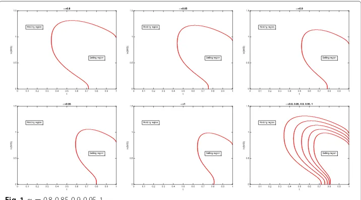
To investigate comparative statics, we present one numerical example in which we change the value of the parameterα. Following the standard approach for estimating the above problem via the finite difference approach, we solve the mathematical formulation given in Eq. (16) by imposing a uniform grid on the(t,y)domain. A Crank-Nicolson scheme is adopted for the discretization of the partial differential equation and the semi-infinite interval foryis truncated at a sufficiently large value ofy. The derivative boundary condi-tion is discretized using a forward difference approximacondi-tion. For the results shown below, we take the grid spacing to be 0.005 foryand 0.001 fortdimensions.

Letm=3. The interest rate of the bond and the appreciation rate of themstocks are

r=0.05 and(b1,b2,b3)=(0.1, 0.12, 0.15), respectively, and the volatility matrix is

σ =

⎡ ⎢ ⎣

0.3000 0 0 0.2000 0.3464 0 0.2500 0.1443 0.4082

⎤ ⎥ ⎦.

Then

θ :=σ−1(b1−r,b2−r,b3−r)=(0.1667, 0.1058, 0.1055).

Using Theorem 1 and the parameter value ofαranging between 0.8 and 1, we observe that the exit region decreases as the value ofα increases, as shown by the combined picture at the right-bottom corner of Fig. 1.

Conclusion

This paper considers an optimal stopping time point for the investor who is expected to maximize her personal utilities and to minimize the difference between the realized return at the stopping point and her potentially maximum return. Our utility function of a quadratic form is more general than that of a fraction form where the denominator may be zero in Shiryaev et al. (2008). Furthermore, our investment problem, which includes the portfolio in the drift and volatility terms of the dynamic systems, makes the problem including multi-dimensional financial assets more realistic and meaningful.

Appendix A: expression of functionG1

We now derive the explicit expression of the functionG1, defined by

G1(t,y) = E

exp

max

y, max

0≤u≤T−t(νu+B(u))

= (_y∞ezdP

max

0≤u≤T−t(νu+B(u))≤z

+eyP

max

0≤u≤T−t(νu+B(u))≤y . Note that P max

0≤u≤T−t(νu+B(u))≤z

=

z−_√ν(T−t)

T−t

−e2νz

−z−_√ν(T−t) T−t

.

According to the standard normal distribution, we have

(∞ y ezd

z−_√ν(T−t)

T−t

= (_y∞ez√ 1 2π(T−t)e

−(z−ν(T−t))2 2(T−t) _dz

= e(ν+1₂)(T−t)₁₋y−(ν_√+1)(T−t) T−t

.

Assume thatν= −1₂. Then

(∞ y ezd

e2νz

−z−_√ν(T−t) T−t

= (_y∞2νe(1+2ν)z−z−_√ν(T−t) T−t

dz+(_y∞e(1+2ν)z_d−z−_√ν(T−t) T−t

= − 2ν 1+2νe

(1+2ν)y−y−_√ν(T−t) T−t

− 1 1+2νe

ν+1₂(T−t)₁₋y−(ν_√+1)(T−t) T−t

.

Thus

G1(t,y) = ey

y−_√ν(T−t) T−t

− 1 1+2νe

(1+2ν)y−y−_√ν(T−t) T−t

+2(1+ν) 1+2ν e

ν+1₂(T−t)₁₋y−(ν_√+1)(T−t) T−t

.

In addition, note that whenν= −1₂,

(_∞ y ezd

e2νz

−z−_√ν(T−t) T−t

= (_y∞ezd

e−z

−z−_√ν(T−t) T−t

= −(_y∞

−z−_√ν(T−t) T−t

dz+(_y∞d

−z−_√ν(T−t) T−t

= y

₋ y−_√ν(T−t)

T−t

− √_√T−t 2π e

−(x+ν(T−t))2

2(T−t) +_ν(T−_t)

1−

y+_√ν(T−t)

T−t

−

₋ y−_√ν(T−t)

T−t

Thus

G1(t,y) = 1−

y−(ν_√+1)(T−t) T−t

−y

₋ y−_√ν(T−t)

T−t

+√_√T−t 2π e

−(y+ν(T−t))2 2(T−t)

−ν(T−t)

1−

y+_√ν(T−t) T−t

+ey

y−_√ν(T−t) T−t

.

Appendix B: expression of functionG2

We now derive the explicit expression of the functionG2, defined by

G2(t,y) = E

exp

max

y, max

0≤u≤T−t(νu+B(u))

2

= (_y∞e2zdP

max

0≤u≤T−t(νu+B(u))≤z

+e2yP

max

0≤u≤T−t(νu+B(u))≤y . Note that P max

0≤u≤T−t(νu+B(u))≤z

=

z−_√ν(T−t) T−t

−e2νz−z−_√ν(T−t) T−t

.

According to the standard normal distribution, we have

(_∞ y e2zd

z−_√ν(T−t)

T−t

= (_y∞e2z√ 1 2π(T−t)e

−(z−ν(T−t))2 2(T−t) _dz

= e2(ν+1)(T−t)

1−

y−(ν_√+2)(T−t) T−t

.

Assume thatν= −1. Then

(∞ y e2zd

e2νz

−z−_√ν(T−t) T−t

= (_y∞2νe2(1+ν)z−z−_√ν(T−t) T−t

dz+(_x∞e2(1+ν)z_d−z−_√ν(T−t) T−t

= − ν 1+νe2

(1+ν)y−y−_√ν(T−t) T−t

− 1 1+νe2

(ν+1)(T−t)₁₋y−(ν_√+2)(T−t) T−t

.

Thus

G2(t,y) = e2y

y−_√ν(T−t) T−t

− 1

1+2νe2(1+ν)y

₋ y−_√ν(T−t)

T−t

+2+ν 1+νe2

(ν+1)(T−t)₁₋y−(ν_√+2)(T−t) T−t

.

Also, note that whenν= −1,

(_∞ y e2zd

e2νz−z−_√ν(T−t) T−t

= (_y∞e2z_de−2z−z−_√ν(T−t) T−t

= −2(_y∞

−z−_√ν(T−t) T−t

dz+(_y∞d

−z−_√ν(T−t) T−t

= 2y

₋ y_√−ν(T−t)

T−t

− 2√_√T−t 2π e

−(y+ν(T−t))2

2(T−t) +_2ν(T−_t)

1−

y+_√ν(T−t) T−t

−

₋ y−_√ν(T−t)

T−t

Thus

G2(t,y) = 1−

y−(ν_√+2)(T−t) T−t

−2y

₋ y−_√ν(T−t)

T−t

+ 2√_√T−t 2π e

−(y+ν(T−t))2 2(T−t)

−2ν(T−t)

1−

y+_√ν(T−t)

T−t

+e2y

y−_√ν(T−t) T−t

.

Funding

This work is supported by Research Grants Council of Hong Kong under grant no. 519913 and 15224215, and National Natural Science Foundation of China (No.11571124).

Authors’ contributions

All authors read and approved the final manuscript.

Competing interests

The authors declare that they have no competing interests.

Publisher’s Note

Springer Nature remains neutral with regard to jurisdictional claims in published maps and institutional affiliations.

Author details

1_{Department of Applied Mathematics, The Hong Kong Polytechnic University, Hong Kong, China.}2_{School of}

Mathematical Sciences, South China Normal University, Guangzhou, China.

Received: 8 October 2017 Accepted: 2 November 2017

References

Ceci C, Bassan B (2004) Mixed optimal stopping and stochastic control problems with semicontinuous final reward for diffusion processes. Stochast Stochast Rep 76:323–337

Chang MH, Pang T, Yong J (2009) Optimal stopping problem for stochastic differential equations with random coefficients. SIAM J Control Optim 48:941–971

Choi K, Koo H, Kwak D (2004) Optimal stopping of active portfolio management. Ann Econ Finance 5:93–126 Dayanik S, Karatzas I (2003) On the optimal stopping problem for one-dimensional diffusions. Stochast Process Appl

107:173–212

Li D, Ng WL (2000) Optimal dynamic portfolio selection: Multi-period means-variance formulation. Math Financ 10:387–406

Li X, Zhou XY (2006) Continuous-time mean-variance efficiency: The 80% rule. Ann Appl Probab 16:1751–1763 Markowitz H (1952) Portfolio selection. J Finance 7:77–91

Markowitz, H (1959) Portfolio Selection: Efticient Diversification of Investments

Merton RC (1969) Lifetime portfolio selection under uncertainty: The continuous-time case. Rev Econ Stat 51:247–257 Merton, RC (1971) Optimum consumption and portfolio rules in a continuous-time model. J Econ Theory 3:373–413 Merton, RC (1973) Theory of rational option pricing. Bell J Econ Manag Sci 4:141–183

Shiryaev A, Xu ZQ, Zhou XY (2008) Thou shalt buy and hold. Quant Finan 8:765–776