Graph Laplacians and their Convergence on Random Neighborhood
Graphs
Matthias Hein MH@TUEBINGEN.MPG.DE
Max Planck Institute for Biological Cybernetics Dept. Sch¨olkopf
Spemannstraße 38 T¨ubingen 72076, Germany
Jean-Yves Audibert AUDIBERT@CERTIS.FR
CERTIS
Ecole Nationale des Ponts et Chauss´ees 19, rue Alfred Nobel - Cit´e Descartes F-77455 Marne-la-Vall´ee cedex 2, France
Ulrike von Luxburg ULRIKE.LUXBURG@TUEBINGEN.MPG.DE
Max Planck Institute for Biological Cybernetics Dept. Sch¨olkopf
Spemannstraße 38 T¨ubingen 72076, Germany
Editor: Sanjoy Dasgupta
Abstract
Given a sample from a probability measure with support on a submanifold in Euclidean space one can construct a neighborhood graph which can be seen as an approximation of the submanifold. The graph Laplacian of such a graph is used in several machine learning methods like semi-supervised learning, dimensionality reduction and clustering. In this paper we determine the pointwise limit of three different graph Laplacians used in the literature as the sample size increases and the neigh-borhood size approaches zero. We show that for a uniform measure on the submanifold all graph Laplacians have the same limit up to constants. However in the case of a non-uniform measure on the submanifold only the so called random walk graph Laplacian converges to the weighted Laplace-Beltrami operator.
Keywords: graphs, graph Laplacians, semi-supervised learning, spectral clustering, dimensional-ity reduction
1. Introduction
• the Laplacian is the generator of the diffusion process (label propagation in semi-supervised learning),
• the eigenvectors of the Laplacian have special geometric properties (motivation for spectral clustering),
• the Laplacian induces an adaptive regularization functional, which adapts to the density and the geometric structure of the data (semi-supervised learning, classification).
If the data lies inRdthe neighborhood graph built from the random sample can be seen as an ap-proximation of the continuous structure. In particular, if the data has support on a low-dimensional submanifold the neighborhood graph is a discrete approximation of the submanifold. In machine learning we are interested in the intrinsic properties and objects of this submanifold. The approxi-mation of the Laplace-Beltrami operator via the graph Laplacian is a very important one since it has numerous applications as we will discuss later.
Approximations of the Laplace-Beltrami operator or related objects have been studied for cer-tain special deterministic graphs. The easiest case is a grid in Rd. In numerics it is standard to approximate the Laplacian with finite-differences schemes on the grid. These can be seen as a spe-cial instances of a graph Laplacian. There convergence for decreasing grid-size follows easily by an argument using Taylor expansions. Another more involved example is the work of Varopoulos (1984), where for a graph generated by anε-packing of a manifold, the equivalence of certain prop-erties of random walks on the graph and Brownian motion on the manifold have been established. The connection between random walks and the graph Laplacian becomes obvious by noting that the graph Laplacian as well as the Laplace-Beltrami operator are the generators of the diffusion process on the graph and the manifold, respectively. In Xu (2004) the convergence of a discrete ap-proximation of the Laplace Beltrami operator for a triangulation of a 2D-surface inR3was shown. However, it is unclear whether the approximation described there can be written as a graph Lapla-cian and whether this result can be generalized to higher dimensions.
In the case where the graph is generated randomly, only first results have been proved so far. The first work on the large sample limit of graph Laplacians has been done by Bousquet et al. (2004). There the authors studied the convergence of the regularization functional induced by the graph Laplacian using the law of large numbers for U -statistics. In a second step taking the limit of the neighborhoodsize h→0, they got p12∇(p2∇)as the effective limit operator inRd. Their result
has recently been generalized to the submanifold case and uniform convergence over the space of H¨older-functions by Hein (2005, 2006). In von Luxburg et al. (2007), the neighborhoodsize h was kept fixed while the large sample limit of the graph Laplacian was considered. In this setting, the authors showed strong convergence results of graph Laplacians to certain integral operators, which imply the convergence of the eigenvalues and eigenfunctions. Thereby showing the consistency of spectral clustering for a fixed neighborhood size.
In contrast to the previous work in this paper we will consider the large sample limit and the limit as the neighborhood size approaches zero simultaneously for a certain class of neighbhorhood graphs. The main emphasis lies on the case where the data generating measure has support on a submanifold ofRd. The bias term, that is the difference between the continuous counterpart of the
isotropic weights and general probability measures. Additionally Lafon showed that the use of data-dependent weights for the graph allows to control the influence of the density. They all show that the bias term converges pointwise if the neighborhood size goes to zero. The convergence of the graph Laplacian towards these continuous averaging operators was left open. This part was first studied by Hein et al. (2005) and Belkin and Niyogi (2005). In Belkin and Niyogi (2005) the convergence was shown for the so called unnormalized graph Laplacian in the case of a uniform probability measure on a compact manifold without boundary and using the Gaussian kernel for the weights, whereas in Hein et al. (2005) the pointwise convergence was shown for the random walk graph Laplacian in the case of general probability measures on non-compact manifolds with boundary using general isotropic data-dependent weights. More recently Gin´e and Koltchinskii (2006) have extended the pointwise convergence for the unnormalized graph Laplacian shown by Belkin and Niyogi (2005) to uniform convergence on compact submanifolds without boundary giving explicit rates. In Singer (2006), see also Gin´e and Koltchinskii (2006), the rate of convergence given by Hein et al. (2005) has been improved in the setting of the uniform measure. In this paper we will study the three most often used graph Laplacians in the machine learning literature and show their pointwise convergence in the general setting of Lafon (2004) and Hein et al. (2005), that is we will in particular consider the case where by using data-dependent weights for the graph we can control the influence of the density on the limit operator.
In Section 2 we introduce the basic framework necessary to define graph Laplacians for general directed weighted graphs and then simplify the general case to undirected graphs. In particular, we define the three graph Laplacians used in machine learning so far, which we call the normalized, the unnormalized and the random walk Laplacian. In Section 3 we introduce the neighborhood graphs studied in this paper, followed by an introduction to the so called weighted Laplace-Beltrami operator, which will turn out to be the limit operator in general. We also study properties of this limit operator and provide insights why and how this operator can be used for semi-supervised learning, clustering and regression. Then finally we present the main convergence result for all three graph Laplacians and give the conditions on the neighborhood size as a function of the sample size necessary for convergence. In Section 4 we illustrate the main result by studying the difference between the three graph Laplacians and the effects of different data-dependent weights on the limit operator. In Section 5 we prove the main result. We introduce a framework for studying non-compact manifolds with boundary and provide the necessary assumptions on the submanifold M, the data generating measure P and the kernel k used for defining the weights of the edges. We would like to note that the theorems given in Section 5 contain slightly stronger results than the ones presented in Section 3. The reader who is not familiar with differential geometry will find a brief introduction to the basic material used in this paper in Appendix A.
2. Abstract Definition of the Graph Structure
In this section we define the structure on a graph which is required in order to define the graph Laplacian. To this end one has to introduce Hilbert spaces HV and HE of functions on the vertices V and edges E, define a difference operator d, and then set the graph Laplacian as∆=d∗d. We
and was generalized to directed graphs by Zhou et al. (2005) for a special choice of HV,HE and d.
To our knowledge the very general setting introduced here has not been discussed elsewhere. In many articles graph Laplacians are used without explicitly mentioning d, HV and HE. This
can be misleading since, as we will show, there always exists a whole family of choices for d, HV
and HE which all yield the same graph Laplacian.
2.1 Hilbert Spaces of Functions on the Vertices V and the Edges E
Let (V,W) be a graph where V denotes the set of vertices with |V|=n and W a positive n×n
similarity matrix, that is wi j≥0,i,j=1, . . . ,n. W need not to be symmetric, that means we consider
the case of a directed graph. The special case of an undirected graph will be discussed in a following section. Let E⊂V×V be the set of edges ei j= (i,j)with wi j>0. ei j is said to be a directed edge
from the vertex i to the vertex j with weight wi j. Moreover, we define the outgoing and ingoing sum
of weights of a vertex i as
diout=1
n n
∑
j=1
wi j, dini =
1
n n
∑
j=1
wji.
We assume that diout+diin>0,i=1, . . . ,n, meaning that each vertex has at least one in- or outgoing
edge. LetR+={x∈R|x≥0}andR∗+={x∈R|x>0}. The inner product on the function space RV is defined as
hf,giV =1
n n
∑
i=1
figiχi,
whereχi= (χout(diout) +χin(diin))withχout:R+→R+ andχin:R+→R+,χout(0) =χin(0) =0
and furtherχout andχinstrictly positive onR∗+.
We also define an inner product on the space of functionsRE on the edges:
hF,GiE = 1
2n2
n
∑
i,j=1
Fi jGi jφ(wi j),
where φ:R+ →R+, φ(0) =0 and φstrictly positive on R∗
+. Note that with these assumptions on φthe sum is taken only over the set of edges E. One can check that both inner products are well-defined. We denote by
H
(V,χ) = (RV,h·,·iV)and
H
(E,φ) = (RE,h·,·iE)the correspondingHilbert spaces. As a last remark let us clarify the roles ofRV andRE. The first one is the space of functions on the vertices and therefore can be regarded as a normal function space. However, elements ofRE can be interpreted as a flow on the edges so that the function value on an edge ei j corresponds to the ”mass” flowing from one vertex i to the vertex j (per unit time).
2.2 The Difference Operator d and its Adjoint d∗
Definition 1 The difference operator d :
H
(V,χ)→H
(E,φ)is defined as follows:∀ei j∈E, (d f)(ei j) =γ(wi j) (f(j)−f(i)),
Remark 2 Note that d is zero on the constant functions as one would expect it from a derivative.
In Zhou et al. (2004) another difference operator d is used:
(d f)(ei j) =γ(wi j)√f(j)
d(j)− f(i)
√
d(i)
. (1)
Note that in Zhou et al. (2004) they have γ(wi j)≡1. This difference operator is in general not zero on the constant functions. This in turn leads to the effect that the associated Laplacian is also not zero on the constant functions. For general graphs without any geometric interpretation this is just a matter of choice. However, the choice of d matters if one wants a consistent continuum limit of the graph. One cannot expect convergence of the graph Laplacian associated to the difference operator d of Equation (1) towards a Laplacian, since as each of the graph Laplacians in the sequence is not zero on the constant functions, also the limit operator will share this property unless
limn→∞d(Xi) =c,∀i=1, . . . ,n, where c is a constant. We derive also the limit operator of the graph Laplacian induced by the difference operator of Equation (1) introduced by Zhou et al. in the machine learning literature and usually denoted as the normalized graph Laplacian in spectral graph theory (Chung, 1997).
Obviously, in the finite case d is always a bounded operator. The adjoint operator d∗:
H
(E,φ)→H
(V,χ)is defined byhd f,uiE=hf,d∗uiV, ∀f∈H(V,χ), u∈
H
(E,φ).Lemma 3 The adjoint d∗:
H
(E,φ)→H
(V,χ)of the difference operator d is explicitly given by:(d∗u)(l) = 1
2χl
1
n n
∑
i=1
γ(wil)uilφ(wil)−1
n n
∑
i=1
γ(wli)uliφ(wli)
. (2)
Proof Using the indicator function f(j) = j=l it is straightforward to derive:
1
nχl(d
∗u)(l) =hd
·=l,uiE =
1 2n2
n
∑
i=1
γ(wil)uilφ(wil)−γ(wli)uliφ(wli),
where we have usedhd ·=l,uiE =2n12∑ n
i,j=1(d ·=l)i jui jφ(wi j).
The first term of the rhs of (2) can be interpreted as the outgoing flow, whereas the second term can be seen as the ingoing flow. The corresponding continuous counterpart of d is the gradient of a function and for d∗ it is the divergence of a vector-field, measuring the infinitesimal difference between in- and outgoing flow.
2.3 The General Graph Laplacian
Definition 4 (graph Laplacian for a directed graph) Given Hilbert spaces
H
(V,χ)and
H
(E,φ)and the difference operator d :H
(V,χ)→H
(E,φ)the graph Laplacian∆:H
(V,χ)→H
(V,χ)is defined asLemma 5 Explicitly,∆:
H
(V,χ)→H
(V,χ)is given as:(∆f)(l) = 1
2χl
1
n n
∑
i=1
γ(wil)2φ(wil) +γ(wli)2φ(wli)
f(l)−f(i)
.
Proof The explicit expression ∆ can be easily derived by plugging the expression of d∗ and d together:
(d∗d f)(l) = 1
2χl
1
n n
∑
i=1
γ(wil)2[f(l)−f(i)]φ(wil)−1
n n
∑
i=1
γ(wli)2[f(i)−f(l)]φ(wli)
= 1
2χl
h
f(l)1
n n
∑
i=1 b
wi j−1 n
n
∑
i=1
f(i)wi jb i,
where we have introducedwbi j= γ(wil)2φ(wil) +γ(wli)2φ(wli)
.
Proposition 6 ∆is self-adjoint and positive semi-definite.
Proof By definition,hf,∆giV =hd f,dgiE =h∆f,giV, andhf,∆fiV =hd f,d fiE≥0.
2.4 The Special Case of an Undirected Graph
In the case of an undirected graph we have wi j =wji, that is whenever there is an edge from i
to j there is an edge with the same value from j to i. This implies that there is no difference between in- and outgoing edges. Therefore, douti ≡diin, so that we will denote the degree function by d with di =1n∑nj=1wi j. The same for the weights in HV, χout≡χin, so that we have only one
functionχ. If one likes to interpret functions on E as flows, it is reasonable to restrict the space
HE
to antisymmetric functions since symmetric functions are associated to flows which transport the same mass from vertex i to vertex j and back. Therefore, as a net effect, no mass is transported at all so that from a physical point of view these functions cannot be observed at all. Since anyway we consider only functions on the edges of the form d f (where f is inHV
) which are by construction antisymmetric, we will not do this restriction explicitly.The adjoint d∗simplifies in the undirected case to
(d∗u)(l) = 1
2χ(dl)
1
n n
∑
i=1
γ(wil)φ(wil)(uil−uli),
and the general graph Laplacian on an undirected graph has the following form:
Definition 7 (graph Laplacian for an undirected graph) Given Hilbert spaces
H
(V,χ)andH
(E,φ)and the difference operator d :H
(V,χ)→H
(E,φ)the graph Laplacian∆:H
(V,χ)→H
(V,χ)is defined as∆=d∗d. Explicitly, for any vertex l, we have
(∆f)(l) = (d∗d f)(l) = 1
χ(dl)
f(l)1
n n
∑
i=1
γ2(wil)φ(wil)−1
n n
∑
i=1
f(i)γ2(wil)φ(wil)
In the literature one finds the following special cases of the general graph Laplacian. Unfortu-nately there exist no unique names for the three graph Laplacians we introduce here, most of the time all of them are just called graph Laplacians. Only the term ’unnormalized’ or ’combinatorial’ graph Laplacian seems to be established now. However, the other two could both be called normal-ized graph Laplacian. Since the first one is closely related to a random walk on the graph we call it random walk graph Laplacian and the other one normalized graph Laplacian.
The ’random walk’ graph Laplacian is defined as:
(∆(rw)f)(i) = f(i)− 1
di
1
n n
∑
j=1
wi jf(j), ∆(rw)f= ( −D−1W)f,
where the matrix D is defined as Di j =diδi j. Note that P=D−1W is a stochastic matrix and
therefore can be used to define a Markov random walk on V , see for example Woess (2000). The ’unnormalized’ (or ’combinatorial’) graph Laplacian is defined as
(∆(u)f)(i) =d
if(i)−
1
n n
∑
j=1
wi jf(j), ∆(u)f = (D−W)f.
We have the following conditions onχ,γandφin order to get these Laplacians:
∀ei j∈E : rw :
γ2(w
i j)φ(wi j)
χ(di) =
wi j
di , unnorm :
γ2(w
i j)φ(wi j)
χ(di) =wi j.
We observe that by choosing ∆(rw) or ∆(u) the functionsφ and γare not fixed. Therefore it can cause confusion if one speaks of the ’random walk’ or ’unnormalized’ graph Laplacian without explicitly defining the corresponding Hilbert spaces and the difference operator. We also consider the normalized graph Laplacian ∆(n) introduced by Chung (1997); Zhou et al. (2004) using the difference operator of Equation (1) and the general spaces H(V,χ) and
H
(E,φ). Following the scheme a straightforward calculation shows the following:Lemma 8 The graph Laplacian∆norm=d∗d with the difference operator d from Equation (1) can
be explicitly written as
(∆(n)f)(l) = 1
nχ(dl)√dl
f(l)
√ dl 1 n n
∑
i=1 γ2(w
il)φ(wil)−
1
n n
∑
i=1
f(i)
√
di
γ2(w
il)φ(wil)
.
The choiceχ(dl) =1 andγ2(wil)φ(wil) =willeads then to the graph Laplacian proposed in Chung and Langlands (1996); Zhou et al. (2004),
(∆(n)f)(l) = 1 n√dl
f(l)
√
dldl−
1
n n
∑
i=1
f(i)
√ diwli =1 n
f(l)−1
n n
∑
i=1
f(i)√wil
dldi
,
or equivalently
∆(n)f =D−1
2(D−W)D−
1
2 f = ( −D−
1
2W D−
1 2)f.
3. Limit of the Graph Laplacian for Random Neighborhood Graphs
Before we state the convergence results for the three graph Laplacians on random neighborhood graphs, we first have to define the limit operator. Maybe not surprisingly, in general the Laplace-Beltrami operator will not be the limit operator of the graph Laplacian. Instead it will converge to the weighted Laplace-Beltrami operator which is the natural generalization of the Laplace-Beltrami operator for a Riemannian manifold equipped with a non-uniform probability measure. The def-inition of this limit operator and a discussion of its use for different applications in clustering, semi-supervised learning and regression is the topic of the next section, followed by a sketch of the convergence results.
3.1 Construction of the Neighborhood Graph
We assume to have a sample Xi,i=1, . . . ,n drawn i.i.d. from a probability measure P which has
support on a submanifold M. For the exact assumptions regarding P, M and the kernel function k used to define the weights we refer to Section 5.2. The sample then determines the set of vertices V of the graph. Additionally we are given a certain kernel function k :R+→R+and the neighborhood parameter h∈R∗+. As proposed by Lafon (2004) and Coifman and Lafon (2006), we use this kernel function k to define the following family of data-dependent kernel functions ˜kλ,hparameterized by λ∈Ras:
˜kλ,h(Xi,Xj) =
1
hm
k(Xi−Xj
2
/h2)
[dh,n(Xi)dh,n(Xj)]λ ,
where dh,n(Xi) = 1n∑ni=1h1mk(
Xi−Xj
2
/h2) is the degree function introduced in Section 2 with respect to the edge-weights h1mk(
Xi−Xj
2
/h2). Finally we use ˜k
λ,h to define the weight wi j = w(Xi,Xj)of the edge between the points Xiand Xjas
wλ,h(Xi,Xj) =˜kλ,h(Xi,Xj).
Note that the caseλ=0 corresponds to weights with no data-dependent modification. The parameter
h∈R∗
+ determines the neighborhood of a point since we will assume that k has compact support, that is Xi and Xj have an edge if
Xi−Xj
≤hRk where Rk is the support of kernel function. Note
that we will have k(0) =0, so that there are no loops in the graph. This assumption is not necessary, but it simplifies the proofs and makes some of the estimators unbiased.
In Section 2.4 we introduced the random walk, the unnormalized and the normalized graph Laplacian. From now on we consider these graph Laplacians for the random neighborhood graph, that is the weights of the graph wi j have the form wi j =w(Xi,Xj) = ˜kλ,h(Xi,Xj). Using the kernel
function we can easily extend the graph Laplacians to the whole submanifold M. These extensions can be seen as estimators for the Laplacian on M. We introduce also the extended degree function
˜
dλ,h,nand the average operator ˜Aλ,h,n,
˜
dλ,h,n(x) =
1
n n
∑
j=1
˜kλ,h(x,Xj), (A˜λ,h,nf)(x) =
1
n n
∑
j=1
Note that ˜dλ,h,n=A˜λ,h,n1. The extended graph Laplacians are defined as follows:
random walk (∆(rw)λ,h,nf)(x) = 1
h2
f−d˜1
λ,h,n
˜
Aλ,h,nf
(x) = 1
h2 ˜
Aλ,h,ng
˜
dλ,h,n
!
(x), (3)
unnormalized (∆(u)λ,h,nf)(x) = 1
h2
˜
dλ,h,nf−A˜λ,h,nf
(x) = 1
h2(A˜λ,h,ng)(x), normalized (∆(n)λ,h,nf)(x) = 1
h2√d˜λ,h,n(x)
˜
dλ,h,n√f˜ dλ,h,n−
˜
Aλ,h,n√˜f dλ,h,n
(x)
= 1
h2√d˜λ,h,n(x)(A˜λ,h,ng0)(x), where we have introduced g(y):= f(x)−f(y) and g0(y):= √˜f(x)
dλ,h,n(x)−
f(y)
√˜
dλ,h,n(y)
. Note that all
extensions reproduce the graph Laplacian on the sample:
(∆f)(i) = (∆f)(Xi) = (∆λ,h,nf)(Xi), ∀i=1, . . . ,n.
The factor 1/h2 arises by introducing a factor 1/h in the weightγof the derivative operator d of the graph. This is necessary since d is supposed to approximate a derivative. Since the Laplacian corresponds to a second derivative we get from the definition of the graph Laplacian a factor 1/h2.
We would like to note that in the case of the random walk and and the normalized graph Lapla-cian the normalization with 1/hm in the weights cancels out, whereas it does not cancel for the
unnormalized graph Laplacian except in the case λ=1/2. The problem here is that in general the intrinsic dimension m of the manifold is unknown. Therefore a normalization with the correct factor h1m is not possible, and in the limit h→0 the estimate of the unnormalized graph Laplacian
will generally either vanish or blow up. The easy way to circumvent this is just to rescale the whole estimate such that 1n∑ni=1d˜λ,h,n(Xi)equals a fixed constant for every n. The disadvantage is that this
method of rescaling introduces a global factor in the limit. A more elegant way might be to simulta-neously estimate the dimension m of the submanifold and use the estimated dimension to calculate the correct normalization factor, see, for example, Hein and Audibert (2005). However, in this work we assume for simplicity that for the unnormalized graph Laplacian the intrinsic dimension m of the submanifold is known. It might be interesting to consider both estimates simultaneously, but we leave this as an open problem.
We will consider in the following the limit h→0, that is the neighborhood of each point Xi
shrinks to zero. However, since n→∞and h as a function of n approaches zero sufficiently slow, the number of points in each neighborhood approaches∞, so that roughly spoken sums approximate the corresponding integrals. This is the basic principle behind our convergence result and is well known in the framework of nonparametric regression (see Gy ¨orfi et al., 2004).
3.2 The Weighted Laplacian and the Continuous Smoothness Functional
The Laplacian is one of the most prominent operators in mathematics. The following general prop-erties are taken from the books of Rosenberg (1997) and B´erard (1986). It occurs in many partial differential equations governing physics, mainly because in Euclidean space it is the only linear second-order differential operator which is translation and rotation invariant. In Euclidean spaceRd
it is defined as∆Rdf =div(grad f) =∑di=1∂2i f.Moreover, for any domainΩ⊆Rdit is a
and satisfies Z
Ωf∆h dx=−
Z
Ωh∇f,∇hidx.
It can be extended to a self-adjoint operator on L2(Ω) in several ways depending on the choice of boundary conditions. For any compact domainΩ(with suitable boundary conditions) it can be shown that ∆has a pure point spectrum and the eigenfunctions are smooth and form a complete orthonormal basis of L2(Ω), see, for example, B´erard (1986).
The Laplace-Beltrami operator on a Riemannian manifold M is the natural equivalent of the Laplacian inRd, defined as
∆Mf =div(grad f) =∇a∇af.
However, the more natural definition is the following. For any f,g∈Cc∞(M), we have
Z
Mf∆h dV
(x) =−
Z
Mh∇f
,∇hidV(x),
where dV=√det g dx is the natural volume element of M. This definition allows easily an extension to the case where we have a Riemannian manifold M with a measure P . In this paper P will be the probability measure generating the data. We assume in the following that P is absolutely continuous wrt the natural volume element dV of the manifold. Its density is denoted by p. Note that the case when the probability measure is absolutely continuous wrt the Lebesgue measure onRd is a special case of our setting.
A recent review article about the weighted Laplace-Beltrami operator is Grigoryan (2006).
Definition 9 (Weighted Laplacian) Let(M,gab)be a Riemannian manifold with measure P where P has a differentiable and positive density p with respect to the natural volume element dV =
√
det g dx, and let∆Mbe the Laplace-Beltrami operator on M. For s∈R, we define the s-th weighted Laplacian∆sas
∆s:=∆M+ s pg
ab(∇
ap)∇b=
1
psg ab∇
a(ps∇b) =
1
psdiv(p sgrad).
This definition is motivated by the following equality, for f,g∈C∞c(M),
Z
M
f(∆sg)psdV = Z
M
f ∆g+s
ph∇p,∇gi
psdV =−
Z
Mh∇
f,∇gipsdV, (4)
The family of weighted Laplacians contains two cases which are particularly interesting. The first one, s=0, corresponds to the standard Laplace-Beltrami operator. This case is interesting if one only wants to use properties of the geometry of the manifold but not of the data generat-ing probability measure. The second case, s=1, corresponds to the standard weighted Laplacian ∆1= 1p∇a(p∇a).
• The Laplacian generates the diffusion process. In semi-supervised learning algorithms with a small number of labeled points one would like to propagate the labels along regions of high-density, see Zhu and Ghahramani (2002); Zhu et al. (2003). The limit operator∆sshows the
influence of a non-uniform density p. The second term sph∇p,∇fileads to an anisotropy in the diffusion. If s<0 this term enforces diffusion in the direction of the maximum of the den-sity whereas diffusion in the direction away from the maximum of the denden-sity is weakened. If s<0 this is just the other way round.
• The smoothness functional induced by the weighted Laplacian∆s, see Equation (4), is given
by
S(f) =
Z
Mk∇
fk2psdV.
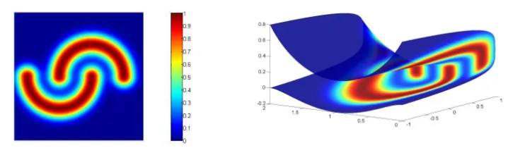
For s>0 this smoothness functional prefers functions which are smooth in high-density re-gions whereas unsmooth behavior in low-density is penalized less. This property can also be interesting in semi-supervised learning where one assumes especially when only a few la-beled points are known that the classifier should be constant in high-density regions whereas changes of the classifier are allowed in low-density regions, see Bousquet et al. (2004) for some discussion of this point and Hein (2005, 2006) for a proof of convergence of the regular-izer induced by the graph Laplacian towards the smoothness functional S(f). In Figure 1 this is illustrated by mapping a density profile inR2onto a two-dimensional manifold. However,
Figure 1: A density profile mapped onto a two-dim. submanifold inR3with two clusters. also the case s<0 can be interesting. Minimizing the smoothness functional S(f)implies that one enforces smoothness of the function f where one has little data, and one allows the function to vary more where one has sampled a lot of data points. Such a penalization has been considered by Canu and Elisseeff (1999) for regression.
• The eigenfunctions of the Laplacian∆s can be seen as the limit partioning of spectral
the eigenfunction corresponding to the first non-zero eigenvalue is likely to change its sign in a low-density region. This argument follows from the previous discussion on the smoothness functional S(f)and the Rayleigh-Ritz principle. Let us assume for a moment that M is com-pact without boundary and that p(x)>0,∀x∈M, then the eigenspace corresponding to the
first eigenvalueλ0=0 is given by the constant functions. The first non-zero eigenvalue can then be determined by the Rayleigh-Ritz variational principle
λ1= inf
u∈C∞(M) R
Mk∇uk
2
p(x)sdV(x) R
Mu2(x)p(x)sdV(x)
Z
M
u(x)p(x)sdV(x) =0
.
Since the first eigenfunction has to be orthogonal to the constant functions, it has to change its sign. However, sincek∇uk2is weighted by a power of the density psit is obvious that for
s>0 the function will change its sign in a region of low density.
3.3 Limit of the Graph Laplacians
The following theorem summarizes and slightly weakens the results of Theorem 30 and Theorem 31 of Section 5.
Main Result Let M be a m-dimensional submanifold inRd,{Xi}n
i=1a sample from a probability
measure P on M with density p. Let x∈M\∂M and define s=2(1−λ). Then under technical conditions on the submanifold M, the kernel k and the density p introduced in Section 5, if h→0
and nhm+2/log n→∞,
random walk: lim
n→∞(∆
(rw)
λ,h,nf)(x) ∼ −(∆sf)(x) almost surely,
unnormalized: lim
n→∞(∆ (u)
λ,h,nf)(x) ∼ −p(x)
1−2λ(∆
sf)(x) almost surely.
The optimal rate is obtained for h(n) =O(log n/n)m1+4
. If h→0 and nhm+4/log n→∞,
normalized: lim
n→∞(∆ (n)
λ,h,nf)(x) ∼ −p(x) 1 2−λ∆s
f
p12−λ
(x) almost surely.
where∼means that there exists a constant only depending on the kernel k andλsuch that equality holds.
the cluster assumption labels in regions of low density are less informative than labels in regions of high density. In general, from the viewpoint of a diffusion process the weighted Laplace-Beltrami operator∆s=∆M+sp∇p∇can be seen as inducing an anisotropic diffusion due to the extra term
s
p∇p∇, which is directed towards or away from increasing density depending on s. This is a desired
property in semi-supervised learning, where one actually wants that the diffusion is mainly along regions of the same density level in order to fulfill the cluster assumption.
The second observation is that the data-dependent modification of edge weights allows to control the influence of the density on the limit operator as observed by Coifman and Lafon (2006). In fact one can even eliminate it for s=0 resp. λ=1 in the case of the random walk graph Laplacian. This could be interesting in computer graphics where the random walk graph Laplacian is used for mesh and point cloud processing, see, for example, Sorkine (2006). If one has gathered points of a curved object with a laser scanner it is likely that the points have a non-uniform distribution on the object. Its surface is a two-dimensional submanifold inR3. In computer graphics the non-uniform measure is only an artefact of the sampling procedure and one is only interested in the Laplace-Beltrami operator to infer geometric properties. Therefore the elimination of the influence of a non-uniform measure on the submanifold is of high interest there. We note that up to a multiplication with the inverse of the density the elimination of density effects is also possible for the unnormalized graph Laplacian, but not for the normalized graph Laplacian. All previous observations are naturally also true if the data does not lie on a submanifold but has d-dimensional support inRd.
The interpretation of the limit of the normalized graph Laplacian is more involved. An expan-sion of the limit operator shows the complex dependency on the density p:
p12−λ∆s
f
p12−λ
=∆Mf+
1
p∇p∇f−(λ−
1 2)
2 f
pk∇pk
2+ (λ −12)f
p∆Mp.
We leave it to the reader to think of possible applications of this Laplacian.
The discussion shows that the choice of the graph Laplacian depends on what kind of problem one wants to solve. Therefore, in our opinion there is no universal best choice between the random walk and the unnormalized graph Laplacian from a machine learning point of view. However, from a mathematical point of view only the random walk graph Laplacian has the correct (pointwise) limit to the weighted Laplace-Beltrami operator.
4. Illustration of the Results
In this section we want to illustrate the differences between the three graph Laplacians and the control of the influence of the data-generating measure via the parameterλ.
4.1 Flat SpaceR2
Figure 2: For the uniform distribution all graph Laplacians, ∆(rw)λ,h,n, ∆(u)λ,h,n and∆(n)λ,h,n (from left to right) agree up to constants for all λ. In the figure the estimates of the Laplacian are shown for the uniform measure on [−3,3]2 and the function f(x) =sin(1
2kxk 2)/
kxk2
with 2500 samples and h=1.4.
in the case ofR2 with a Gaussian distribution
N
(0,1)as data-generating measure and the simple function f(x) =∑ixi−4. Note that∆f=0 so that for the random walk and the unnormalized graphLaplacian only the anisotropic part of the limit operator, 1p∇p∇f is non-zero. Explicitly the limits
are given as
∆(rw)
∼ ∆sf=∆f+ s
p∇p∇f =−s
∑
ixi,∆(u)
∼ p1−2λ∆sf=−s e− 1−2λ
2 kxk 2
∑
ixi,∆(n)
∼ p12−λ∆s f
p12−λ =−
∑
ixi−∑
ixi−4h
(λ−1
2)( 3
2−λ)kxk 2
−2(λ−1
2) i
.
This shows that even applied to simple functions there can be large differences between the different limit operators provided the samples come from a non-uniform probability measure. Note that like in nonparametric kernel regression the estimate is quite bad at the boundary. This well known boundary effect arises since at the boundary one does not average over a full ball but only over some part of a ball. Thus the first derivative∇f of order O(h)does not cancel out so that multiplied with the factor 1/h2we have a term of order O(1/h) which blows up. Roughly spoken this effect takes place at all points of order O(h)away from the boundary, see also Coifman and Lafon (2006).
4.2 The Sphere S2
In our next example we consider the case where the data lies on a submanifold M in Rd. Here
we want to illustrate in the case of a sphere S2 inR3 the control of the influence of the density via the parameterλ. In this case we sample from the probability measure with density p(φ,θ) =
1 8π+
3
Figure 3: Illustration of the differences of the three graph Laplacians, random walk, unnormalized and normalized (from the top) forλ=0. The function f is f =∑2
i=1xi−4 and the 2500
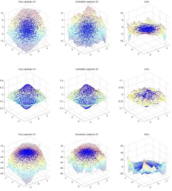
random walk graph Laplacian together with the result of the weighted Laplace-Beltrami operator and an error plot forλ=0,1,2 resulting in s=−2,0,2 for the function f(φ,θ) =cos(θ). First one can see that for a non-uniform probability measure the results for different values ofλdiffer quite a lot. Note that the function f is adapted to the cluster structure in the sense that it does not change much in each cluster but changes very much in region of low density. In the case of s=2 we can see that∆sf would lead to a diffusion which would lead roughly to a kind of step function which
changes at the equator. The same is true for s=0 but the effect is much smaller than for s=2. In the case of s=−2 we have a completely different behavior.∆sf has now flipped its sign near to the
equator so that the induced diffusion process would try to smooth the function in the low density region.
5. Proof of the Main Result
In this section we will present the main results which were sketched in Section 3.3 together with the proofs. In Section 5.1 we first introduce some non-standard tools from differential geometry which we will use later on. In particular, it turns out that the so called manifolds with boundary of bounded geometry are the natural framework where one can still deal with non-compact manifolds in a setting comparable to the compact case. After a proper statement of the assumptions under which we prove the convergence results of the graph Laplacian and a preliminary result about convolutions on submanifolds which is of interest on its own, we then start with the final proofs. The proof is basically divided into two parts, the bias and the variance, where these terms are only approximately valid. The reader not familiar with differential geometry is encouraged to first read the appendix on basics of differential geometry in order to be equipped with the necessary background.
5.1 Non-compact Submanifolds inRdwith Boundary
We prove the pointwise convergence for non-compact submanifolds. Therefore we have to restrict the class of submanifolds since manifolds with unbounded curvature do not allow reasonable func-tion spaces.
Remark 10 In the rest of this paper we use the Einstein summation convention that is over indices
occurring twice has to be summed. Note that the definition of the curvature tensor differs between textbooks. We use here the conventions regarding the definitions of curvature etc. of Lee (1997).
5.1.1 MANIFOLDS WITHBOUNDARY OFBOUNDEDGEOMETRY
−1 0 1 −0.50 0.5 −1 0 1 f −0.5 0 0.5 −1 0 1 −0.50 0.5 −1 0 1 Density 0 0.01 0.02 0.03 0.04 0.05 −1 0 1 −0.50 0.5 −1 0 1
True Laplacian of f
−1 0 1 −1 0 1 −0.50 0.5 −1 0 1
Estimated Laplacian of f
−1 0 1 −1 0 1 −0.50 0.5 −1 0 1 error −1 0 1 2 −1 0 1 −0.50 0.5 −1 0 1
True Laplacian of f
−1 0 1 −1 0 1 −0.50 0.5 −1 0 1
Estimated Laplacian of f
−1 0 1 −1 0 1 −0.50 0.5 −1 0 1 error −1 0 1 2 −1 0 1 −0.50 0.5 −1 0 1
True Laplacian of f
−2 0 2 −1 0 1 −0.50 0.5 −1 0 1
Estimated Laplacian of f
−2 0 2 −1 0 1 −0.50 0.5 −1 0 1 error −2 −1 0 1 2
Figure 4: Illustration of the effect ofλ=0,1,2 (row 2−4) resulting in s=−2,0,2 for the sphere with a non-uniform data-generating probability measure and the function f(θ,φ) =cos(θ)
Note that the boundary∂M is an isometric submanifold of M of dimension m−1. Therefore it has a second fundamental formΠwhich should not be mixed up with the second fundamental form Πof M which is with respect to the ambient spaceRd. We denote by∇the connection and by R the curvature of∂M. Moreover, letνbe the normal inward vector field at∂M.
Definition 11 (Manifold with boundary of bounded geometry) Let M be a manifold with
bound-ary∂M (possibly empty). It is of bounded geometry if the following holds:
• (N) Normal Collar: there exists rC>0 so that the normal geodesic flow,
K :(x,t)→expx(tνx),
is defined on∂M×[0,rC) and is a diffeomorphism onto its image (νx is the inward normal vector). Let N(s):=K(∂M×[0,s])be the collar set for 0≤s≤rC.
• (IC) The injectivity radius inj∂M of∂M is positive.
• (I) Injectivity radius of M: There is ri>0 so that if r≤rithen for x∈M\N(r)the exponential map is a diffeomorphism on BM(0,r)⊂TxM so that normal coordinates are defined on every ball BM(x,r)for x∈M\N(r).
• (B) Curvature bounds: For every k∈N there is Ck so that |∇iR| ≤Ck and ∇iΠ≤Ck for 0≤i≤k, where∇i denotes the covariant derivative of order i.
Note that(B)imposes bounds on all orders of the derivatives of the curvatures. One could also restrict the definition to the order of derivatives needed for the goals one pursues. But this would require even more notational effort, therefore we skip this. In particular, in Schick (1996) it is argued that boundedness of all derivatives of the curvature is very close to the boundedness of the curvature alone.
The lower bound on the injectivity radius of M and the bound on the curvature are standard to define manifolds of bounded geometry without boundary. Now the problem of the injectivity radius of M is that at the boundary it somehow makes only partially sense since injM(x)→0 as
d(x,∂M)→0. Therefore one replaces next to the boundary standard normal coordinates with normal collar coordinates.
Definition 12 (normal collar coordinates) Let M be a Riemannian manifold with
boundary∂M. Fix x0∈∂M and an orthonormal basis of Tx0∂M to identify Tx0∂M withRm−1. For
r1,r2>0 sufficiently small (such that the following map is injective) define normal collar
coordi-nates,
nx0 : BRm−1(0,r1)×[0,r2]→M :(v,t)→expM
exp∂x0M(v)(tν). The pair(r1,r2)is called the width of the normal collar chart nx0.
The next proposition shows why manifolds of bounded geometry are especially interesting.
• (B1) There exist 0<R1≤rinj(∂M), 0<R2≤rC and 0<R3≤ri and constants CK>0 for
each K∈Nsuch that whenever we have normal boundary coordinates of width(r1,r2)with r1≤R1and r2≤R2or normal coordinates of radius r3≤rithen in these coordinates,
|Dαgi j| ≤CK and |Dαgi j| ≤CK for all |α| ≤K.
The condition(B)in Definition 11 holds if and only if(B1)holds. The constants CKcan be chosen to depend only on ri,rC,inj∂Mand Ck.
Note that due to gi jgjk=δik one gets upper and lower bounds on the operator norms of g and g−1, respectively, which result in upper and lower bounds for √det g. This implies that we have upper and lower bounds on the volume form dV(x) =√det g dx.
Lemma 14 (Schick 2001) Let(M,g)be a Riemannian manifold with boundary of
bounded geometry of dimension m. Then there exists R0>0 and constants S1>0 and S2such that
for all x∈M and r≤R0one has
S1rm≤vol(BM(x,r))≤S2rm.
Another important tool for analysis on manifolds are appropriate function spaces. In order to define a Sobolev norm one first has to fix a family of charts Ui with M⊂ ∪iUi and then define
the Sobolev norm with respect to these charts. The resulting norm will depend on the choice of the charts Ui. Since in differential geometry the choice of the charts should not matter, the natural
question arises how the Sobolev norm corresponding to a different choice of charts Vi is related to
that for the choice Ui. In general, the Sobolev norms will not be the same. However, if one assumes
that the transition maps are smooth and the manifold M is compact then the resulting norms will be equivalent and therefore define the same topology. Now if one has a non-compact manifold this argumentation does not work anymore. This problem is solved in general by defining the norm with respect to a covering of M by normal coordinate charts. Then it can be shown that the change of coordinates between these normal coordinate charts is well-behaved due to the bounded geometry of M. In that way it is possible to establish a well-defined notion of Sobolev spaces on manifolds with boundary of bounded geometry in the sense that any norm defined with respect to a different covering of M by normal coordinate charts is equivalent. Let(Ui,φi)i∈Ibe a countable covering of
the submanifold M with normal coordinate charts of M, that is M⊂ ∪i∈IUi, then:
kfkCk(M)=max
m≤ksupi∈I x∈supφ
i(Ui)
Dm(f◦φ−1
i )(x)
.
In the following we will denote with Ck(M)the space of Ck-functions on M together with the norm k·kCk(M).
5.1.2 INTRINSIC VERSUSEXTRINSICPROPERTIES
Most of the proofs for the continuous part will work with Taylor expansions in normal coordinates. It is then of special interest to have a connection between intrinsic and extrinsic distances. Since the distance on M is induced fromRd, it is obvious that one haskx−yk
Rd ∼dM(x,y) for all x,y∈M
the neighborhood of a point x∈M. Particularly, it gives a third-order approximation of the intrinsic
distance dM(x,y)in M in terms of the extrinsic distance in the ambient space X which is in our case
just the Euclidean distance inRd.
Proposition 15 Let i : M→Rd be an isometric embedding of the smooth m-dimensional Rieman-nian manifold M intoRd. Let x∈M and V be a neighborhood of 0 inRmand letΨ: V→U provide normal coordinates of a neighborhood U of x, that isΨ(0) =x. Then for all y∈V :
kyk2Rm=dM2(x,Ψ(y)) =k(i◦Ψ)(y)−i(x)k2+
1
12kΠ(γ˙,γ˙)k 2
TxRd+O(kyk
5
Rm),
whereΠis the second fundamental form of M andγthe unique geodesic from x toΨ(y)such that
˙
γ=yi∂yi. The volume form dV =pdet gi j(y)dy of M satisfies in normal coordinates,
dV =1+1
6Riuviy
uyv+O(
kyk3Rm)
dy,
In particular,
(∆pdet gi j)(0) =−
1 3R,
where R is the scalar curvature (i.e., R=gikgjlRi jkl).
We would like to note that in Smolyanov, von Weizs¨acker, and Wittich (2007) this proposition was formulated for general ambient spaces X , that is arbitrary Riemannian manifolds X . Using the more general form of this proposition one could extend the results in this paper to submanifolds of other ambient spaces X . However, in order to use the scheme one needs to know the geodesic distances in X , which are usually not available for general Riemannian manifolds. Nevertheless, for some special cases like the sphere, one knows the geodesic distances. Submanifolds of the sphere could be of interest, for example in geophysics or astronomy.
The previous proposition is very helpful since it gives an asymptotic expression of the geodesic distance dM(x,y)on M in terms of the extrinsic Euclidean distance. The following lemma is a
non-asymptotic statement taken from Bernstein et al. (2001) which we present in a slightly different form. But first we establish a connection between what they call the ’minimum radius of curvature’ and upper bounds on the extrinsic curvatures of M and∂M. Let
Πmax=sup
x∈M
sup
v∈TxM,kvk=1
kΠ(v,v)k, Πmax= sup
x∈∂M
sup
v∈Tx∂M,kvk=1
Π(v,v),
whereΠis the second fundamental form of∂M as a submanifold of M. We set Πmax=0 if the boundary∂M is empty.
Using the relation between the acceleration in the ambient space and the second fundamental form for unit-speed curvesγwith no acceleration in M (Dt˙γ=0) established in Section A.3, we get
for the Euclidean acceleration of such a curveγinRd,
k¨γk=kΠ(˙γ,˙γ)k.
Now if one has a non-empty boundary∂M it can happen that a length-minimizing curve goes
is Dtc˙=∇c˙c˙=0 where∇is the connection of∂M induced by M. However, c will not be a geodesic in M (in the sense of a curve with no acceleration) since by the Gauss-Formula in Theorem 41,
Dtc˙=Dtc˙+Π(c,˙ c˙) =Π(c,˙ c˙).
Therefore, in general the upper bound on the Euclidean acceleration of a length-minimizing curveγ in M is given by,
kγ¨k=Π(γ˙,γ˙) +Π(γ˙,γ˙)≤Πmax+Πmax.
Using this inequality, one can derive a lower bound on the ’minimum radius of curvature’ρdefined in Bernstein et al. (2001) as ρ=inf{1/kγ¨kRd} where the infimum is taken over all unit-speed
geodesicsγof M (in the sense of length-minimizing curves):
ρ≥Π 1
max+Πmax
.
Finally we can formulate the Lemma from Bernstein et al. (2001).
Lemma 16 Let x,y∈M with dM(x,y)≤πρ. Then
2ρsin(dM(x,y)/(2ρ))≤ kx−ykRd ≤dM(x,y).
Noting that sin(x)≥x/2 for 0≤x≤π/2, we get as an easier to handle corollary:
Corollary 17 Let x,y∈M with dM(x,y)≤πρ. Then
1
2dM(x,y)≤ kx−ykRd ≤dM(x,y).
In the given form this corollary is quite useless since we only have the Euclidean distances between points and therefore we have no possibility to check the condition dM(x,y)≤πρ. In general
small Euclidean distance does not imply small intrinsic distance. Imagine a circle where one has cut out a very small segment. Then the Euclidean distance between the two ends is very small however the geodesic distance is very large. We show now that under an additional assumption one can transform the above corollary so that one can use it when one has only knowledge about Euclidean distances.
Lemma 18 Let M have a finite radius of curvatureρ>0. We further assume that,
κ:= inf
x∈My∈M\infBM(x,πρ)
kx−yk,
is non-zero. Then BRd(x,κ/2)∩M⊂BM(x,κ)⊂BM(x,πρ). Particularly, if x,y∈M andkx−yk ≤
κ/2, then
1
2dM(x,y)≤ kx−ykRd ≤dM(x,y)≤κ.
Proof By definitionκis at most the infimum ofkx−ykwhere y satisfies dM(x,y) =πρ. Therefore
the set BRd(x,κ/2)∩M is a subset of BM(x,πρ). The rest of the lemma then follows by Corollary
Figure 5: κis the Euclidean distance of x∈M to M\BM(x,πρ).
5.2 Notations and Assumptions
In general we work on complete non-compact manifolds with boundary. Compared to a setting where one considers only compact manifolds one needs a slightly larger technical overhead. How-ever, we will indicate how the technical assumptions simplify if one has a compact submanifold with boundary or even a compact manifold without boundary.
We impose the following assumptions on the manifold M:
Assumption 19 (i) The map i : M→Rdis a smooth embedding,
(ii) The manifold M with the metric induced from Rd is a smooth manifold with boundary of bounded geometry (possibly∂M=/0),
(iii) M has bounded second fundamental form,
(iv) It holdsκ:=infx∈Minfy∈M\BM(x,πρ)ki(x)−i(y)k>0, whereρis the radius of curvature defined
in Section 5.1.2,
(v) For any x∈M\∂M, δ(x):= inf
y∈M\BM(x,31min{inj(x),πρ})
ki(x)−i(y)kRd >0,where inj(x) is the
injectivity radius1at x andρ>0 is the radius of curvature.
The first condition ensures that i(M)is a smooth submanifold ofRd. Usually we do not distin-guish between i(M)and M. The use of the abstract manifold M as a starting point emphasizes that there exists an m-dimensional smooth manifold M or roughly equivalent an m-dimensional smooth parameter space underlying the data. The choice of the d features determines then the representa-tion inRd. The choice of features corresponds therefore to a specific choice of the inclusion map i since i determines how M is embedded intoRd. This means that another choice of features leads in general to a different mapping i but the initial abstract manifold M is always the same. However, in the second condition we assume that the metric structure of M is induced byRd(which implies that i is trivially an isometric embedding). Therefore the metric structure depends on the embedding i or
equivalently on our choice of features.
The second condition ensures that M is an isometric submanifold ofRdwhich is well-behaved. As discussed in Section 5.1.1, manifolds of bounded geometry are in general non-compact, complete Riemannian manifolds with boundary where one has uniform control over all intrinsic curvatures. The uniform bounds on the curvature allow to do reasonable analysis in this general setting. In
particular, it allows us to introduce the function spaces Ck(M)with their associated norm. It might be possible to prove pointwise results even without the assumption of bounded geometry. But we think that the setting studied here is already general enough to encompass all cases encountered in practice.
The third condition ensures that M also has well-behaved extrinsic geometry and implies that the radius of curvatureρis lower bounded. Together with the fourth condition it enables us to get global upper and lower bounds of the intrinsic distance on M in terms of the extrinsic distance in Rdand vice versa, see Lemma 18.
The fourth condition is only necessary in the case of non-compact submanifolds. It prevents the manifold from self-approaching. More precisely it ensures that if parts of M are far away from x in the geometry of M they do not come too close to x in the geometry ofRd. Assuming that i(M)is a submanifold, this assumption is already included implicitly. However, for non-compact subman-ifolds the self-approaching could happen at infinity. Therefore we exclude it explicitly. Moreover, note that for submanifolds with boundary one has inj(x)→0 as x approaches the boundary2 ∂M.
Therefore alsoδ(x)→0 as d(x,∂M)→0. However, this behavior ofδ(x)at the boundary does not matter for the proof of pointwise convergence in the interior of M.
Note that if M is a smooth and compact manifold conditions (ii)-(v) hold automatically. In order to emphasize the distinction between extrinsic and intrinsic properties of the manifold we always use the slightly cumbersome notations x∈M (intrinsic) and i(x)∈Rd (extrinsic). The reader who is not familiar with Riemannian geometry should keep in mind that locally, a subman-ifold of dimension m looks likeRm. This becomes apparent if one uses normal coordinates. Also the following dictionary between terms of the manifold M and the case when one has only an open set inRd(i is then the identity mapping) might be useful.
Manifold M open set inRd gi j,√det g δi j , 1
natural volume element Lebesgue measure ∆s ∆s=∑di=1 ∂
2
∂(zi)2+
s p∑
d i=1∂∂zpi∂∂zi
The kernel functions which are used to define the weights of the graph are always functions of the squared norm inRd. Furthermore, we make the following assumptions on the kernel function k:
Assumption 20 (i) k :R+→Ris measurable, non-negative and non-increasing onR∗+,
(ii) k∈C2(R∗+), that is in particular k, ∂k
∂x and ∂ 2k
∂x2 are bounded,
(iii) k,|∂∂kx|and|∂∂2xk2|have exponential decay: ∃c,α,A∈R+such that for any t≥A, f(t)≤ce−αt, where f(t) =max{k(t),|∂k
∂x|(t),|∂ 2k
∂x2|(t)},
(iv) k(0) =0.
The assumption that the kernel is non-increasing could be dropped, however it makes the proof and the presentation easier. Moreover, in practice the weights of the neighborhood graph which are determined by k are interpreted as similarities. Therefore the usual choice is to take weights which