Evolutionary Function Approximation
for Reinforcement Learning
Shimon Whiteson [email protected]
Peter Stone [email protected]
Department of Computer Sciences University of Texas at Austin 1 University Station, C0500 Austin, TX 78712-0233
Editor: Georgios Theocharous
Abstract
Temporal difference methods are theoretically grounded and empirically effective methods for ad-dressing reinforcement learning problems. In most real-world reinforcement learning tasks, TD methods require a function approximator to represent the value function. However, using function approximators requires manually making crucial representational decisions. This paper investi-gates evolutionary function approximation, a novel approach to automatically selecting function approximator representations that enable efficient individual learning. This method evolves indi-viduals that are better able to learn. We present a fully implemented instantiation of evolutionary function approximation which combines NEAT, a neuroevolutionary optimization technique, with Q-learning, a popular TD method. The resulting NEAT+Q algorithm automatically discovers ef-fective representations for neural network function approximators. This paper also presents on-line
evolutionary computation, which improves the on-line performance of evolutionary computation
by borrowing selection mechanisms used in TD methods to choose individual actions and using them in evolutionary computation to select policies for evaluation. We evaluate these contributions with extended empirical studies in two domains: 1) the mountain car task, a standard reinforcement learning benchmark on which neural network function approximators have previously performed poorly and 2) server job scheduling, a large probabilistic domain drawn from the field of autonomic computing. The results demonstrate that evolutionary function approximation can significantly prove the performance of TD methods and on-line evolutionary computation can significantly im-prove evolutionary methods. This paper also presents additional tests that offer insight into what factors can make neural network function approximation difficult in practice.
Keywords: reinforcement learning, temporal difference methods, evolutionary computation,
neu-roevolution, on-line learning
1. Introduction
The most common approach to reinforcement learning relies on the concept of value functions, which indicate, for a particular policy, the long-term value of a given state or state-action pair.
Tem-poral difference methods (TD) (Sutton, 1988), which combine principles of dynamic programming
with statistical sampling, use the immediate rewards received by the agent to incrementally improve both the agent’s policy and the estimated value function for that policy. Hence, TD methods en-able an agent to learn during its “lifetime” i.e. from its individual experience interacting with the environment.
For small problems, the value function can be represented as a table. However, the large, proba-bilistic domains which arise in the real-world usually require coupling TD methods with a function
approximator, which represents the mapping from state-action pairs to values via a more concise,
parameterized function and uses supervised learning methods to set its parameters. Many different methods of function approximation have been used successfully, including CMACs, radial basis functions, and neural networks (Sutton and Barto, 1998). However, using function approxima-tors requires making crucial representational decisions (e.g. the number of hidden units and ini-tial weights of a neural network). Poor design choices can result in estimates that diverge from the optimal value function (Baird, 1995) and agents that perform poorly. Even for reinforcement learning algorithms with guaranteed convergence (Baird and Moore, 1999; Lagoudakis and Parr, 2003), achieving high performance in practice requires finding an appropriate representation for the function approximator. As Lagoudakis and Parr observe, “The crucial factor for a successful ap-proximate algorithm is the choice of the parametric approximation architecture(s) and the choice of the projection (parameter adjustment) method.” (Lagoudakis and Parr, 2003, p. 1111) Nonetheless, representational choices are typically made manually, based only on the designer’s intuition.
Our goal is to automate the search for effective representations by employing sophisticated op-timization techniques. In this paper, we focus on using evolutionary methods (Goldberg, 1989) because of their demonstrated ability to discover effective representations (Gruau et al., 1996; Stan-ley and Miikkulainen, 2002). Synthesizing evolutionary and TD methods results in a new approach called evolutionary function approximation, which automatically selects function approximator rep-resentations that enable efficient individual learning. Thus, this method evolves individuals that are better able to learn. This biologically intuitive combination has been applied to computational sys-tems in the past (Hinton and Nowlan, 1987; Ackley and Littman, 1991; Boers et al., 1995; French and Messinger, 1994; Gruau and Whitley, 1993; Nolfi et al., 1994) but never, to our knowledge, to aid the discovery of good TD function approximators.
Our approach requires only 1) an evolutionary algorithm capable of optimizing representations from a class of functions and 2) a TD method that uses elements of that class for function ap-proximation. This paper focuses on performing evolutionary function approximation with neural networks. There are several reasons for this choice. First, they have great experimental value. Non-linear function approximators are often the most challenging to use; hence, success for evolutionary function approximation with neural networks is good reason to hope for success with linear methods too. Second, neural networks have great potential, since they can represent value functions linear methods cannot (given the same basis functions). Finally, employing neural networks is feasible because they have previously succeeded as TD function approximators (Crites and Barto, 1998; Tesauro, 1994) and sophisticated methods for optimizing their representations (Gruau et al., 1996; Stanley and Miikkulainen, 2002) already exist.
TD method. The resulting algorithm, called NEAT+Q, uses NEAT to evolve topologies and initial weights of neural networks that are better able to learn, via backpropagation, to represent the value estimates provided by Q-learning.
Evolutionary computation is typically applied to off-line scenarios, where the only goal is to discover a good policy as quickly as possible. By contrast, TD methods are typically applied to
on-line scenarios, in which the agent tries to learn a good policy quickly and to maximize the reward it
obtains while doing so. Hence, for evolutionary function approximation to achieve its full potential, the underlying evolutionary method needs to work well on-line.
TD methods excel on-line because they are typically combined with action selection
mecha-nisms likeε-greedy and softmax selection (Sutton and Barto, 1998). These mechanisms improve
on-line performance by explicitly balancing two competing objectives: 1) searching for better poli-cies (exploration) and 2) gathering as much reward as possible (exploitation). This paper investi-gates a novel approach we call on-line evolutionary computation, in which selection mechanisms commonly used by TD methods to choose individual actions are used in evolutionary computation to choose policies for evaluation. We present two implementations, based onε-greedy and softmax selection, that distribute evaluations within a generation so as to favor more promising individu-als. Since on-line evolutionary computation can be used in conjunction with evolutionary function approximation, the ability to optimize representations need not come at the expense of the on-line aspects of TD methods. On the contrary, the value function and its representation can be optimized simultaneously, all while the agent interacts with its environment.
We evaluate these contributions with extended empirical studies in two domains: 1) mountain car and 2) server job scheduling. The mountain car task (Sutton and Barto, 1998) is a canonical reinforcement learning benchmark domain that requires function approximation. Though the task is simple, previous researchers have noted that manually designed neural network function approxi-mators are often unable to master it (Boyan and Moore, 1995; Pyeatt and Howe, 2001). Hence, this domain is ideal for a preliminary evaluation of NEAT+Q.
Server job scheduling (Whiteson and Stone, 2004), is a large, probabilistic reinforcement learn-ing task from the field of autonomic computlearn-ing (Kephart and Chess, 2003). In server job schedullearn-ing, a server, such as a website’s application server or database, must determine in what order to process a queue of waiting jobs so as to maximize the system’s aggregate utility. This domain is challenging because it is large (the size of both the state and action spaces grow in direct proportion to the size of the queue) and probabilistic (the server does not know what type of job will arrive next). Hence, it is a typical example of a reinforcement learning task that requires effective function approximation. Using these domains, our experiments test Q-learning with a series of manually designed neu-ral networks and compare the results to NEAT+Q and regular NEAT (which trains action selectors in lieu of value functions). The results demonstrate that evolutionary function approximation can significantly improve the performance of TD methods. Furthermore, we test NEAT and NEAT+Q
with and withoutε-greedy and softmax versions of evolutionary computation. These experiments
confirm that such techniques can significantly improve the on-line performance of evolutionary computation. Finally, we present additional tests that measure the effect of continual learning on function approximators. The results offer insight into why certain methods outperform others in these domains and what factors can make neural network function approximation difficult in prac-tice.
manually. Second, it provides an objective analysis of the strengths and weaknesses of evolutionary and TD methods, opportunistically combining the strengths into a single approach. Though the TD and evolutionary communities are mostly disjoint and focus on somewhat different problems, we find that each can benefit from the progress of the other. On the one hand, we show that methods for evolving neural network topologies can find TD function approximators that perform better. On the other hand, we show that established techniques from the TD community can make evolutionary methods applicable to on-line learning problems.
The remainder of this paper is organized as follows. Section 2 provides background on Q-learning and NEAT, the constituent Q-learning methods used in this paper. Section 3 introduces the novel methods and details the particular implementations we tested. Section 4 describes the moun-tain car and server job scheduling domains and Section 5 presents and discusses empirical results. Section 7 overviews related work, Section 8 outlines opportunities for future work, and Section 9 concludes.
2. Background
We begin by reviewing Q-learning and NEAT, the algorithms that form the building blocks of our implementations of evolutionary function approximation.
2.1 Q-Learning
There are several different TD methods currently in use, including Q-learning (Watkins, 1989), Sarsa (Sutton and Barto, 1998), and LSPI (Lagoudakis and Parr, 2003). The experiments presented in this paper use Q-learning because it is a well-established, canonical method that has also enjoyed empirical success, particularly when combined with neural network function approximators (Crites and Barto, 1998). We present it as a representative method but do not claim it is superior to other TD approaches. In principle, evolutionary function approximation can be used with any of them. For example, many of the experiments described in Section 5 have been replicated with Sarsa (Sutton and Barto, 1998), another popular TD method, in place of Q-learning, yielding qualitatively similar results.
Like many other TD methods, Q-learning attempts to learn a value function Q(s,a)that maps state-action pairs to values. In the tabular case, the algorithm is defined by the following update rule, applied each time the agent transitions from state s to state s′:
Q(s,a)←(1−α)Q(s,a) +α(r+γmaxa′Q(s′,a′))
whereα∈[0,1]is a learning rate parameter,γ∈[0,1]is a discount factor, and r is the immediate reward the agent receives upon taking action a.
output better matches the current value estimate for the state-action pair: r+γmaxa′Q(s′,a′). The
adjustments are made via theBACKPROPfunction, which implements the standard backpropagation
algorithm (Rumelhart et al., 1986) with the addition of accumulating eligibility traces controlled by
λ(Sutton and Barto, 1998). The agent usesε-greedy selection (Sutton and Barto, 1998) to ensure it occasionally tests alternatives to its current policy (lines 10–11). The agent interacts with the environment via theTAKE-ACTIONfunction (line 15), which returns a reward and a new state.
Algorithm 1Q-LEARN(S,A,σ,c,α,γ,λ,εtd,e)
1: // S: set of all states, A: set of all actions,σ: standard deviation of initial weights
2: // c: output scale,α: learning rate,γ: discount factor,λ: eligibility decay rate
3: //εtd: exploration rate, e: total number of episodes 4:
5: N←INIT-NET(S,A,σ) // make a new network N with random weights
6: for i←1 to e do
7: s,s′←null,INIT-STATE(S) // environment picks episode’s initial state
8: repeat
9: Q[]←c×EVAL-NET(N,s′) // compute value estimates for current state
10: with-prob(εtd) a′←RANDOM(A) // select random exploratory action
11: else a′←argmaxjQ[j] // or select greedy action
12: if s6=null then
13: BACKPROP(N,s,a,(r+γmaxjQ[j])/c,α,γ,λ) // adjust weights toward target 14: s,a←s′,a′
15: r,s′←TAKE-ACTION(a′) // take action and transition to new state 16: untilTERMINAL-STATE?(s)
2.2 NEAT1
The implementation of evolutionary function approximation presented in this paper relies on Neu-roEvolution of Augmenting Topologies (NEAT) to automate the search for appropriate topologies and initial weights of neural network function approximators. NEAT is an appropriate choice be-cause of its empirical successes on difficult reinforcement learning tasks like non-Markovian double pole balancing (Stanley and Miikkulainen, 2002), game playing (Stanley and Miikkulainen, 2004b), and robot control (Stanley and Miikkulainen, 2004a), and because of its ability to automatically op-timize network topologies.
In a typical neuroevolutionary system (Yao, 1999), the weights of a neural network are strung together to form an individual genome. A population of such genomes is then evolved by evaluating each one and selectively reproducing the fittest individuals through crossover and mutation. Most neuroevolutionary systems require the designer to manually determine the network’s topology (i.e. how many hidden nodes there are and how they are connected). By contrast, NEAT automatically evolves the topology to fit the complexity of the problem. It combines the usual search for network weights with evolution of the network structure.
NEAT is an optimization technique that can be applied to a wide variety of problems. Section 3 below describes how we use NEAT to optimize the topology and initial weights of TD function
approximators. Here, we describe how NEAT can be used to tackle reinforcement learning problems without the aid of TD methods, an approach that serves as one baseline of comparison in Section 5. For this method, NEAT does not attempt to learn a value function. Instead, it finds good policies directly by training action selectors, which map states to the action the agent should take in that state. Hence it is an example of policy search reinforcement learning. Like other policy search methods, e.g. (Sutton et al., 2000; Ng and Jordan, 2000; Mannor et al., 2003; Kohl and Stone, 2004), it uses global optimization techniques to directly search the space of potential policies.
Algorithm 2NEAT(S,A,p,mn,ml,g,e)
1: // S: set of all states, A: set of all actions, p: population size, mn: node mutation rate 2: // ml: link mutation rate, g: number of generations, e: episodes per generation
3:
4: P[]←INIT-POPULATION(S,A,p) // create new population P with random networks
5: for i←1 to g do
6: for j←1 to e do
7: N,s,s′←RANDOM(P[]), null,INIT-STATE(S) // select a network randomly
8: repeat
9: Q[]←EVAL-NET(N,s′) // evaluate selected network on current state
10: a′←argmaxiQ[i] // select action with highest activation
11: s,a←s′,a′
12: r,s′←TAKE-ACTION(a′) // take action and transition to new state
13: N.f itness←N.f itness+r // update total reward accrued by N
14: untilTERMINAL-STATE?(s)
15: N.episodes←N.episodes+1 // update total number of episodes for N
16: P′[]←new array of size p // new array will store next generation
17: for j←1 to p do
18: P′[j]←BREED-NET(P[]) // make a new network based on fit parents in P
19: with-probability mn:ADD-NODE-MUTATION(P′[j]) // add a node to new network 20: with-probability ml:ADD-LINK-MUTATION(P′[j]) // add a link to new network 21: P[]←P′[]
Algorithm 2 contains a high-level description of the NEAT algorithm applied to an episodic reinforcement learning problem. This implementation differs slightly from previous versions of NEAT in that evaluations are conducted by randomly selecting individuals (line 7), instead of the more typical approach of stepping through the population in a fixed order. This change does not significantly alter NEAT’s behavior but facilitates the alterations we introduce in Section 3.2. During each step, the agent takes whatever action corresponds to the output with the highest activation (lines 10–12). NEAT maintains a running total of the reward accrued by the network during its evaluation (line 13). Each generation ends after e episodes, at which point each network’s average fitness is
2.2.1 MINIMIZINGDIMENSIONALITY
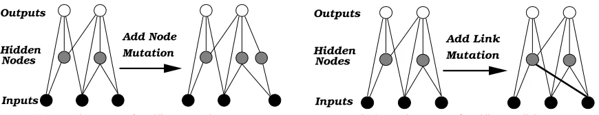
Unlike other systems that evolve network topologies and weights (Gruau et al., 1996; Yao, 1999) NEAT begins with a uniform population of simple networks with no hidden nodes and inputs con-nected directly to outputs. New structure is introduced incrementally via two special mutation operators. Figure 1 depicts these operators, which add new hidden nodes and links to the network. Only the structural mutations that yield performance advantages tend to survive evolution’s selec-tive pressure. In this way, NEAT tends to search through a minimal number of weight dimensions and find an appropriate complexity level for the problem.
Inputs Nodes Hidden Outputs
00000000000000 11111111111111
Mutation Add Node
Inputs Nodes Hidden Outputs
Mutation Add Link
(a) A mutation operator for adding new nodes (b) A mutation operator for adding new links
Figure 1: Examples of NEAT’s mutation operators for adding structure to networks. In (a), a hidden node is added by splitting a link in two. In (b), a link, shown with a thicker black line, is added to connect two nodes.
2.2.2 GENETICENCODING WITHHISTORICALMARKINGS
Evolving network structure requires a flexible genetic encoding. Each genome in NEAT includes a list of connection genes, each of which refers to two node genes being connected. Each con-nection gene specifies the in-node, the out-node, the weight of the concon-nection, whether or not the connection gene is expressed (an enable bit), and an innovation number, which allows NEAT to find corresponding genes during crossover.
In order to perform crossover, the system must be able to tell which genes match up between any individuals in the population. For this purpose, NEAT keeps track of the historical origin of every gene. Whenever a new gene appears (through structural mutation), a global innovation number is incremented and assigned to that gene. The innovation numbers thus represent a chronology of every gene in the system. Whenever these genomes crossover, innovation numbers on inherited genes are preserved. Thus, the historical origin of every gene in the system is known throughout evolution.
Through innovation numbers, the system knows exactly which genes match up with which. Genes that do not match are either disjoint or excess, depending on whether they occur within or outside the range of the other parent’s innovation numbers. When crossing over, the genes in both genomes with the same innovation numbers are lined up. Genes that do not match are inherited from the more fit parent, or if they are equally fit, from both parents randomly.
2.2.3 SPECIATION
In most cases, adding new structure to a network initially reduces its fitness. However, NEAT speciates the population, so that individuals compete primarily within their own niches rather than with the population at large. Hence, topological innovations are protected and have time to optimize their structure before competing with other niches in the population.
Historical markings make it possible for the system to divide the population into species based on topological similarity. The distanceδbetween two network encodings is a simple linear combi-nation of the number of excess (E) and disjoint (D) genes, as well as the average weight differences of matching genes (W ):
δ= c1E
N +
c2D
N +c3·W
The coefficients c1, c2, and c3adjust the importance of the three factors, and the factor N, the number
of genes in the larger genome, normalizes for genome size. Genomes are tested one at a time; if a genome’s distance to a randomly chosen member of the species is less than δt, a compatibility
threshold, it is placed into this species. Each genome is placed into the first species where this condition is satisfied, so that no genome is in more than one species.
The reproduction mechanism for NEAT is explicit fitness sharing (Goldberg and Richardson, 1987), where organisms in the same species must share the fitness of their niche, preventing any one species from taking over the population.
3. Method
This section describes evolutionary function approximation and a complete implementation called NEAT+Q. It also describes on-line evolutionary computation and details two ways of implementing it in NEAT+Q.
3.1 Evolutionary Function Approximation
When evolutionary methods are applied to reinforcement learning problems, they typically evolve a population of action selectors, each of which remains fixed during its fitness evaluation. The central insight behind evolutionary function approximation is that, if evolution is directed to evolve value functions instead, then those value functions can be updated, using TD methods, during each fitness evaluation. In this way, the system can evolve function approximators that are better able to learn via TD.
In addition to automating the search for effective representations, evolutionary function approx-imation can enable synergistic effects between evolution and learning. How these effects occur depends on which of two possible approaches is employed. The first possibility is a Lamarckian approach, in which the changes made by TD during a given generation are written back into the original genomes, which are then used to breed a new population. The second possibility is a
Dar-winian implementation, in which the changes made by TD are discarded and the new population is
bred from the original genomes, as they were at birth.
learn-ing. However, Darwinian evolution can be advantageous because it enables each generation to reproduce the genomes that led to success in the previous generation, rather than relying on altered versions that may not thrive under continued alteration. Furthermore, in a Darwinian system, the learning conducted by previous generations can be indirectly recorded in a population’s genomes via a phenomenon called the Baldwin Effect (Baldwin, 1896), which has been demonstrated in evo-lutionary computation (Hinton and Nowlan, 1987; Ackley and Littman, 1991; Boers et al., 1995; Arita and Suzuki, 2000). The Baldwin Effect occurs in two stages. In the first stage, the learning performed by individuals during their lifetimes speeds evolution, because each individual does not have to be exactly right at birth; it need only be in the right neighborhood and learning can adjust it accordingly. In the second stage, those behaviors that were previously learned during individu-als’ lifetimes become known at birth. This stage occurs because individuals that possess adaptive behaviors at birth have higher overall fitness and are favored by evolution.
Hence, synergistic effects between evolution and learning are possible regardless of which im-plementation is used. In Section 5, we compare the two approaches empirically. The remainder of this section details NEAT+Q, the implementation of evolutionary function approximation used in our experiments.
3.1.1 NEAT+Q
All that is required to make NEAT optimize value functions instead of action selectors is a rein-terpretation of its output values. The structure of neural network action selectors (one input for each state feature and one output for each action) is already identical to that of Q-learning function approximators. Therefore, if the weights of the networks NEAT evolves are updated during their fitness evaluations using Q-learning and backpropagation, they will effectively evolve value func-tions instead of action selectors. Hence, the outputs are no longer arbitrary values; they represent the long-term discounted values of the associated state-action pairs and are used, not just to select the most desirable action, but to update the estimates of other state-action pairs.
Algorithm 3 summarizes the resulting NEAT+Q method. Note that this algorithm is identical to Algorithm 2, except for the delineated section containing lines 13–16. Each time the agent takes an action, the network is backpropagated towards Q-learning targets (line 16) andε-greedy selection occurs just as in Algorithm 1 (lines 13–14). Ifαandεtd are set to zero, this method degenerates to
regular NEAT.
NEAT+Q combines the power of TD methods with the ability of NEAT to learn effective rep-resentations. Traditional neural network function approximators put all their eggs in one basket by relying on a single manually designed network to represent the value function. NEAT+Q, by con-trast, explores the space of such networks to increase the chance of finding a representation that will perform well.
Algorithm 3NEAT+Q(S,A,c,p,mn,ml,g,e,α,γ,λ,εtd)
1: // S: set of all states, A: set of all actions, c: output scale, p: population size
2: // mn: node mutation rate, ml: link mutation rate, g: number of generations
3: // e: number of episodes per generation,α: learning rate,γ: discount factor
4: //λ: eligibility decay rate,εtd: exploration rate 5:
6: P[]←INIT-POPULATION(S,A,p) // create new population P with random networks
7: for i←1 to g do
8: for j←1 to e do
9: N,s,s′←RANDOM(P[]), null,INIT-STATE(S) // select a network randomly
10: repeat
11: Q[]←c×EVAL-NET(N,s′) // compute value estimates for current state 12:
13: with-prob(εtd) a′←RANDOM(A) // select random exploratory action
14: else a′←argmaxkQ[k] // or select greedy action
15: if s6=null then
16: BACKPROP(N,s,a,(r+γmaxkQ[k])/c,α,γ,λ) // adjust weights toward target 17:
18: s,a←s′,a′
19: r,s′←TAKE-ACTION(a′) // take action and transition to new state
20: N.f itness←N.f itness+r // update total reward accrued by N
21: untilTERMINAL-STATE?(s)
22: N.episodes←N.episodes+1 // update total number of episodes for N
23: P′[]←new array of size p // new array will store next generation
24: for j←1 to p do
25: P′[j]←BREED-NET(P[]) // make a new network based on fit parents in P
3.2 On-Line Evolutionary Computation
To excel in on-line scenarios, a learning algorithm must effectively balance two competing objec-tives. The first objective is exploration, in which the agent tries alternatives to its current best policy in the hopes of improving it. The second objective is exploitation, in which the agent follows the current best policy in order to maximize the reward it receives. TD methods excel at on-line tasks because they are typically combined with action selection mechanisms that achieve this balance (e.g
ε-greedy and softmax selection).
Evolutionary methods, though lacking explicit selection mechanisms, do implicitly perform this balance. In fact, in one of the earliest works on evolutionary computation, Holland (1975) argues that the reproduction mechanism encourages exploration, since crossover and mutation result in novel genomes, but also encourages exploitation, since each new generation is based on the fittest members of the last one. However, reproduction allows evolutionary methods to balance exploration and exploitation only across generations, not within them. Once the members of each generation have been determined, they all typically receive the same evaluation time, even if some individuals dramatically outperform others in early episodes. Hence, within a generation, a typical evolutionary method is purely exploratory, as it makes no effort to favor those individuals that have performed well so far.
Therefore, to excel on-line, evolutionary methods need a way to limit the exploration that occurs within each generation and force more exploitation. In a sense, this problem is the opposite of that faced by TD methods, which naturally exploit (by following the greedy policy) and thus need a way to force more exploration. Nonetheless, the ultimate goal is the same: a proper balance between the two extremes. Hence, we propose that the solution can be the same too. In this section, we discuss ways of borrowing the action selection mechanisms traditionally used in TD methods and applying them in evolutionary computation.
To do so, we must modify the level at which selection is performed. Evolutionary algorithms cannot perform selection at the level of individual actions because, lacking value functions, they have no notion of the value of individual actions. However, they can perform selection at the level of evaluations, in which entire policies are assessed holistically. The same selection mechanisms used to choose individual actions in TD methods can be used to select policies for evaluation, an approach we call on-line evolutionary computation. Using this technique, evolutionary algorithms can excel on-line by balancing exploration and exploitation within and across generations.
The remainder of this section presents two implementations. The first, which relies onε-greedy selection, switches probabilistically between searching for better policies and re-evaluating the best known policy to garner maximal reward. The second, which relies on softmax selection, dis-tributes evaluations in proportion to each individual’s estimated fitness, thereby focusing on the most promising individuals and increasing the average reward accrued.
3.2.1 USING
ε
-GREEDYSELECTION INEVOLUTIONARYCOMPUTATIONWhen ε-greedy selection is used in TD methods, a single parameter, εtd, is used to control what
fraction of the time the agent deviates from greedy behavior. Each time the agent selects an action, it chooses probabilistically between exploration and exploitation. With probabilityεtd, it will explore
by selecting randomly from the available actions. With probability 1−εtd, it will exploit by selecting
In evolutionary computation, this same mechanism can be used to determine which policies to evaluate within each generation. With probabilityεec, the algorithm explores by behaving exactly
as it would normally: selecting a policy for evaluation, either randomly or by iterating through the population. With probability 1−εec, the algorithm exploits by selecting the best policy discovered
so far in the current generation. The score of each policy is just the average reward per episode it has received so far. Each time a policy is selected for evaluation, the total reward it receives is incorporated into that average, which can cause it to gain or lose the rank of best policy.
To applyε-greedy selection to NEAT and NEAT+Q, we need only alter the assignment of the
candidate policy N in lines 7 and 9 of Algorithms 2 and 3, respectively. Instead of a random selection, we use the result of the ε-greedy selection function described in Algorithm 4, where
N.average=N.f itness/N.episodes. In the case of NEAT+Q, two differentεparameters control exploration throughout the system: εtd controls the exploration that helps Q-learning estimate the
value function and εec controls exploration that helps NEAT discover appropriate topologies and
initial weights for the neural network function approximators.
Algorithm 4ε-GREEDY SELECTION(P,εec) 1: // P: population,εec: NEAT’s exploration rate 2:
3: with-prob(εec) returnRANDOM(P) // select random network
4: else return N∈P| ∀(N′∈P)N.average≥N′.average // or select champion
Using ε-greedy selection in evolutionary computation allows it to thrive in on-line scenarios by balancing exploration and exploitation. For the most part, this method does not alter evolu-tion’s search but simply interleaves it with exploitative episodes that increase average reward during learning. The next section describes how softmax selection can be applied to evolutionary compu-tation to intelligently focus search with each generation and create a more nuanced balance between exploration and exploitation.
3.2.2 USINGSOFTMAXSELECTION INEVOLUTIONARYCOMPUTATION
When softmax selection is used in TD methods, an action’s probability of selection is a function of its estimated value. In addition to ensuring that the greedy action is chosen most often, this technique focuses exploration on the most promising alternatives. There are many ways to implement softmax selection but one popular method relies on a Boltzmann distribution (Sutton and Barto, 1998), in which case an agent in state s chooses an action a with probability
eQ(s,a)/τ ∑b∈AeQ(s,b)/τ
where A is the set of available actions, Q(s,a)is the agent’s value estimate for the given state-action pair andτ is a positive parameter controlling the degree to which actions with higher values are favored in selection. The higher the value ofτ, the more equiprobable the actions are.
probabil-ity
eS(p)/τ ∑q∈PeS(q)/τ
where S(p)is the average fitness of the policy p.
To apply softmax selection to NEAT and NEAT+Q, we need only alter the assignment of the candidate policy N in lines 7 and 9 of Algorithms 2 and 3, respectively. Instead of a random se-lection, we use the result of the softmax selection function shown in Algorithm 5. In the case of NEAT+Q,εtd controls Q-learning’s exploration andτcontrols NEAT’s exploration. Of course,
soft-max exploration could be used within Q-learning too. However, since comparing different selection mechanisms for TD methods is not the subject of our research, in this paper we use onlyε-greedy selection with TD methods.
Algorithm 5SOFTMAX SELECTION(P,τ)
1: // P: population,τ: softmax temperature
2:
3: if∃N∈P|N.episodes=0 then
4: return N // give each network one episode before using softmax
5: else
6: total←∑N∈PeN.average/τ // compute denominator of Boltzmann function 7: for all N∈P do
8: with-prob(eN.averagetotal /τ) return N // select N for evaluation
9: else total←total−eN.average/τ // or skip N and reweight probabilities
In addition to providing a more nuanced balance between exploration and exploitation, soft-max selection also allows evolutionary computation to more effectively focus its search within each generation. Instead of spending the same number of evaluations on each member of the popula-tion, softmax selection can quickly abandon poorly performing policies and spend more episodes evaluating the most promising individuals.
In summary, on-line evolutionary computation enables the use of evolutionary computation dur-ing an agent’s interaction with the world. Therefore, the ability of evolutionary function approxima-tion to optimize representaapproxima-tions need not come at the expense of the on-line aspects of TD methods. On the contrary, the value function and its representation can be optimized simultaneously, all while the agent interacts with its environment.
4. Experimental Setup
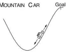
Figure 2: The Mountain Car Task. This figure was taken from Sutton and Barto (1998).
4.1 Mountain Car
In the mountain car task (Boyan and Moore, 1995), depicted in Figure 2, an agent strives to drive a car to the top of a steep mountain. The car cannot simply accelerate forward because its engine is not powerful enough to overcome gravity. Instead, the agent must learn to drive backwards up the hill behind it, thus building up sufficient inertia to ascend to the goal before running out of speed.
The agent’s state at timestep t consists of its current position pt and its current velocity vt.
It receives a reward of -1 at each time step until reaching the goal, at which point the episode terminates. The agent’s three available actions correspond to the throttle settings 1,0, and -1. The following equations control the car’s movement:
pt+1=boundp(pt+vt+1)
vt+1=boundv(vt+0.001at−0.0025cos(3pt))
where atis the action the agent takes at timestep t, boundpenforces−1.2≤pt+1≤0.5, and boundv
enforces−0.07≤vt+1≤0.07. In each episode, the agent begins in a state chosen randomly from
these ranges. To prevent episodes from running indefinitely, each episode is terminated after 2,500 steps if the agent still has not reached the goal.
Though the agent’s state has only two features, they are continuous and hence learning the value function requires a function approximator. Previous research has demonstrated that TD methods can solve the mountain car task using several different function approximators, including CMACs (Sut-ton, 1996; Kretchmar and Anderson, 1997), locally weighted regression (Boyan and Moore, 1995), decision trees (Pyeatt and Howe, 2001), radial basis functions (Kretchmar and Anderson, 1997), and instance-based methods (Boyan and Moore, 1995). By giving the learner a priori knowledge about the goal state and using methods based on experience replay, the mountain car problem has been solved with neural networks too (Reidmiller, 2005). However, the task remains notoriously difficult for neural networks, as several researchers have noted that value estimates can easily diverge (Boyan and Moore, 1995; Pyeatt and Howe, 2001).
We hypothesized that the difficulty of using neural networks in this task is due at least in part to the problem of finding an appropriate representation. Hence, as a preliminary evaluation of evolutionary function approximation, we applied NEAT+Q to the mountain car task to see if it could learn better than manually designed networks. The results are presented in Section 5.
if the agent’s current state fell in that region, and to zero otherwise. Hence, only two inputs were activated for any given state. The networks have three outputs, each corresponding to one of the actions available to the agent.
4.2 Server Job Scheduling
While the mountain car task is a useful benchmark, it is a very simple domain. To assess whether our methods can scale to a much more complex problem, we use a challenging reinforcement learning task called server job scheduling. This domain is drawn from the burgeoning field of autonomic computing (Kephart and Chess, 2003). The goal of autonomic computing is to develop computer systems that automatically configure themselves, optimize their own behavior, and diagnose and repair their own failures. The demand for such features is growing rapidly, since computer systems are becoming so complex that maintaining them with human support staff is increasingly infeasible. The vision of autonomic computing poses new challenges to many areas of computer science, including architecture, operating systems, security, and human-computer interfaces. However, the burden on artificial intelligence is especially great, since intelligence is a prerequisite for self-managing systems. In particular, we believe machine learning will play a primary role, since com-puter systems must be adaptive if they are to perform well autonomously. There are many ways to apply supervised methods to autonomic systems, e.g. for intrusion detection (Ertoz et al., 2004), spam filtering (Dalvi et al., 2004), or system configuration (Wildstrom et al., 2005). However, there are also many tasks where no human expert is available and reinforcement learning is applicable, e.g network routing (Boyan and Littman, 1994), job scheduling (Whiteson and Stone, 2004), and cache allocation (Gomez et al., 2001).
One such task is server job scheduling, in which a server, such as a website’s application server or database, must determine in what order to process the jobs currently waiting in its queue. Its goal is to maximize the aggregate utility of all the jobs it processes. A utility function (not to be confused with a TD value function) for each job type maps the job’s completion time to the utility derived by the user (Walsh et al., 2004). The problem of server job scheduling becomes challenging when these utility functions are nonlinear and/or the server must process multiple types of jobs. Since selecting a particular job for processing necessarily delays the completion of all other jobs in the queue, the scheduler must weigh difficult trade-offs to maximize aggregate utility. Also, this domain is challenging because it is large (the size of both the state and action spaces grow in direct proportion to the size of the queue) and probabilistic (the server does not know what type of job will arrive next). Hence, it is a typical example of a reinforcement learning task that requires effective function approximation.
The server job scheduling task is quite different from traditional scheduling tasks (Zhang and Dietterich, 1995; Zweben and Fox, 1998). In the latter case, there are typically multiple resources available and each job has a partially ordered list of resource requirements. Server job scheduling is simpler because there is only one resource (the server) and all jobs are independent of each other. However, it is more complex in that performance is measured via arbitrary utility functions, whereas traditional scheduling tasks aim solely to minimize completion times.
-160 -140 -120 -100 -80 -60 -40 -20 0
0 50 100 150 200
Utility
Completion Time Utility Functions for All Four Job Types
Job Type #2
Job Type #3
Job Type #4
Job Type #1
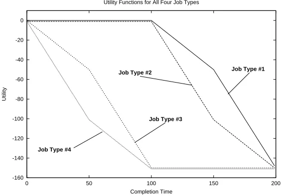
Figure 3: The four utility functions used in our experiments.
decisions about which job to process next even as new jobs are arriving. Since one job is processed at each timestep, each episode lasts 200 timesteps. For each job that completes, the scheduling agent receives an immediate reward determined by that job’s utility function.
Four different job types were used in our experiments. Hence, the task can generate 4200unique episodes. Utility functions for the four job types are shown in Figure 3. Users who create jobs of type #1 or #2 do not care about their jobs’ completion times so long as they are less than 100 timesteps. Beyond that, they get increasingly unhappy. The rate of this change differs between the two types and switches at timestep 150. Users who create jobs of type #3 or #4 want their jobs completed as quickly as possible. However, once the job becomes 100 timesteps old, it is too late to be useful and they become indifferent to it. As with the first two job types, the slopes for job types #3 and #4 differ from each other and switch, this time at timestep 50. Note that all these utilities are negative functions of completion time. Hence, the scheduling agent strives to bring aggregate utility as close to zero as possible.
A primary obstacle to applying reinforcement learning methods to this domain is the size of the state and action spaces. A complete state description includes the type and age of each job in the queue. The scheduler’s actions consist of selecting jobs for processing; hence a complete action space includes every job in the queue. To render these spaces more manageable, we discretize them. The range of job ages from 0 to 200 is divided into four sections and the scheduler is told, at each timestep, how many jobs in the queue of each type fall in each range, resulting in 16 state features. The action space is similarly discretized. Instead of selecting a particular job for processing, the scheduler specifies what type of job it wants to process and which of the four age ranges that job should lie in, resulting in 16 distinct actions. The server processes the youngest job in the queue that matches the type and age range specified by the action.
of the utility function, not the utility function itself, which determines how much utility is lost by delaying a given job.
Even after discretization, the state space is quite large. If the queue holds at most qmax jobs, qmax+1
16
is a loose upper bound on the number of states, since each job can be in one of 16 buckets. Some of these states will not occur (e.g. ones where all the jobs in the queue are in the youngest age range). Nonetheless, with 16 actions per state, it is clearly infeasible to represent the value function in a table. Hence, success in this domain requires function approximation, as addressed in the following section.
5. Results
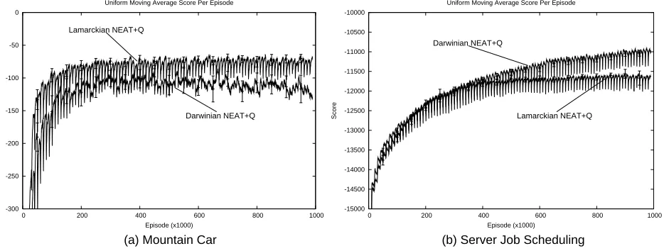
We conducted a series of experiments in the mountain car and server job scheduling domains to empirically evaluate the methods presented in this paper. Section 5.1 compares manual and evo-lutionary function approximators. Section 5.2 compares off-line and on-line evoevo-lutionary compu-tation. Section 5.3 tests evolutionary function approximation combined with on-line evolutionary computation. Section 5.4 compares these novel approaches to previous learning and non-learning methods. Section 5.5 compares Darwinian and Lamarckian versions of evolutionary function ap-proximation. Finally, Section 5.6 presents some addition tests that measure the effect of continual learning on function approximators. The results offer insight into why certain methods outperform others in these domains and what factors can make neural network function approximation difficult in practice.
Each of the graphs presented in these sections include error bars indicating 95% confidence intervals. In addition, to assess statistical significance, we conducted Student’s t-tests on each pair of methods evaluated. The results of these tests are summarized in Appendix A.
5.1 Comparing Manual and Evolutionary Function Approximation
As an initial baseline, we conducted, in each domain, 25 runs in which NEAT attempts to discover a good policy using the setup described in Section 4. In these runs, the population size p was 100, the number of generations g was 100, the node mutation rate mn was 0.02, the link mutation rate
ml was 0.1, and the number of episodes per generation e was 10,000. Hence, each individual was
evaluated for 100 episodes on average. See Appendix B for more details on the NEAT parameters used in our experiments.
Next, we performed 25 runs in each domain using NEAT+Q, with the same parameter settings. The eligibility decay rate λwas 0.0. and the learning rateαwas set to 0.1 and annealed linearly for each member of the population until reaching zero after 100 episodes.2 In scheduling, γwas 0.95 and εtd was 0.05. Those values of γ andεtd work well in mountain car too, though in the
experiments presented here they were set to 1.0 and 0.0 respectively, since Sutton (1996) found that discounting and exploration are unnecessary in mountain car. The output scale c was set to -100 in mountain car and -1000 in scheduling.
We tested both Darwinian and Lamarckian NEAT+Q in this manner. Both perform well, though which is preferable appears to be domain dependent. For simplicity, in this section and those that follow, we present results only for Darwinian NEAT+Q. In Section 5.5 we present a comparison of the two approaches.
To test Q-learning without NEAT, we tried 24 different configurations in each domain. These configurations correspond to every possible combination of the following parameter settings. The networks had feed-forward topologies with 0, 4, or 8 hidden nodes. The learning rateαwas either 0.01 or 0.001. The annealing schedules forαwere linear, decaying to zero after either 100,000 or 250,000 episodes. The eligibility decay rateλwas either 0.0 or 0.6. The other parameters,γand
ε, were set just as with NEAT+Q, and the standard deviation of initial weights σwas 0.1. Each of these 24 configurations was evaluated for 5 runs. In addition, we experimented informally with higher and lower values ofα, higher values of γ, slower linear annealing, exponential annealing, and no annealing at all, though none performed as well as the results presented here.
In these experiments, each run used a different set of initial weights. Hence, the resulting performance of each configuration, by averaging over different initial weight settings, does not account for the possibility that some weight settings perform consistently better than others. To address this, for each domain, we took the best performing configuration3 and randomly selected five fixed initial weight settings. For each setting, we conducted 5 additional runs. Finally, we took the setting with the highest performance and conducted an additional 20 runs, for a total of 25. For simplicity, the graphs that follow show only this Q-learning result: the best configuration with the best initial weight setting.
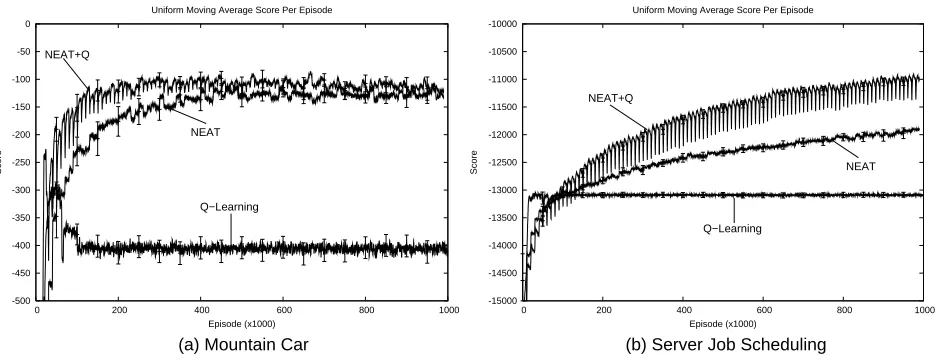
Figure 4 shows the results of these experiments. For each method, the corresponding line in the graph represents a uniform moving average over the aggregate utility received in the past 1,000 episodes, averaged over all 25 runs. Using average performance, as we do throughout this paper, is somewhat unorthodox for evolutionary methods, which are more commonly evaluated on the per-formance of the generation champion. There are two reasons why we adopt average perper-formance. First, it creates a consistent metric for all the methods tested, including the TD methods that do not use evolutionary computation and hence have no generation champions. Second, it is an on-line metric because it incorporates all the reward the learning system accrues. Plotting only generation champions is an implicitly off-line metric because it does not penalize methods that discover good policies but fail to accrue much reward while learning. Hence, average reward is a better metric for evaluating on-line evolutionary computation, as we do in Section 5.2.
To make a larger number of runs computationally feasible, both NEAT and NEAT+Q were run for only 100 generations. In the scheduling domain, neither method has completely plateaued by this point. However, a handful of trials conducted for 200 generations verified that only very small additional improvements are made after 100 generation, without a qualitative effect on the results.
Note that the progress of NEAT+Q consists of a series of 10,000-episode intervals. Each of these intervals corresponds to one generation and the changes within them are due to learning via Q-learning and backpropagation. Although each individual learns for only 100 episodes on average, NEAT’s system of randomly selecting individuals for evaluation causes that learning to be spread across the entire generation: each individual changes gradually during the generation as it is repeat-edly evaluated. The result is a series of intra-generational learning curves within the larger learning curve.
For the particular problems we tested and network configurations we tried, evolutionary func-tion approximafunc-tion significantly improves performance over manually designed networks. In the scheduling domain, Q-learning learns much more rapidly in the very early part of learning. In both domains, however, Q-learning soon plateaus while NEAT and NEAT+Q continue to improve. Of
-15000 -14500 -14000 -13500 -13000 -12500 -12000 -11500 -11000 -10500 -10000
0 200 400 600 800 1000
Score
Episode (x1000) Uniform Moving Average Score Per Episode
-500 -450 -400 -350 -300 -250 -200 -150 -100 -50 0
0 200 400 600 800 1000
Score
Episode (x1000) Uniform Moving Average Score Per Episode
(a) Mountain Car (b) Server Job Scheduling
NEAT+Q NEAT Q−Learning Q−Learning NEAT NEAT+Q
Figure 4: A comparison of the performance of manual and evolutionary function approximators in the mountain car and server job scheduling domains.
course, after 100,000 episodes, Q-learning’s learning rateαhas annealed to zero and no additional
learning is possible. However, its performance plateaus well before α reaches zero and, in our
experiments, running Q-learning with slower annealing or no annealing at all consistently led to inferior and unstable performance.
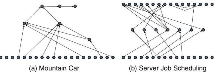
Nonetheless, the possibility remains that additional engineering of the network structure, the feature set, or the learning parameters would significantly improve Q-learning’s performance. In particular, when Q-learning is started with one of the best networks discovered by NEAT+Q and the learning rate is annealed aggressively, Q-learning matches NEAT+Q’s performance without directly using evolutionary computation. However, it is unlikely that a manual search, no matter how extensive, would discover these successful topologies, which contain irregular and partially connected hidden layers. Figure 5 shows examples of typical networks evolved by NEAT+Q.
NEAT+Q also significantly outperforms regular NEAT in both domains. In the mountain car domain, NEAT+Q learns faster, achieving better performance in earlier generations, though both plateau at approximately the same level. In the server job scheduling domain, NEAT+Q learns more rapidly and also converges to significantly higher performance. This result highlights the value of TD methods on challenging reinforcement learning problems. Even when NEAT is employed to find effective representations, the best performance is achieved only when TD methods are used to estimate a value function. Hence, the relatively poor performance of Q-learning is not due to some weakness in the TD methodology but merely to the failure to find a good representation.
Figure 5: Typical examples of the topologies of the best networks evolved by NEAT+Q in both the mountain car and scheduling domains. Input nodes are on the bottom, hidden nodes in the middle, and output nodes on top. In addition to the links shown, each input node is directly connected to each output node. Note that two output nodes can be directly connected, in which case the activation of one node serves not only as an output of the network, but as an input to the other node.
5.2 Comparing Off-Line and On-Line Evolutionary Computation
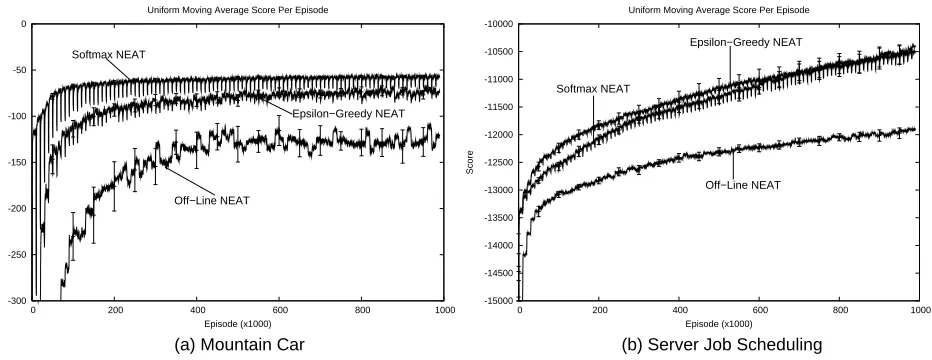
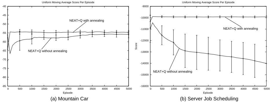
In this section, we present experiments evaluating line evolutionary computation. Since on-line evolutionary computation does not depend on evolutionary function approximation, we first test it using regular NEAT, by comparing an off-line version to on-line versions using ε-greedy and softmax selection. In Section 5.3 we study the effect of combining NEAT+Q with on-line evolutionary computation.
Figure 6 compares the performance of off-line NEAT to its on-line counterparts in both domains. The results for off-line NEAT are the same as those presented in Figure 4. To test on-line NEAT withε-greedy selection, 25 runs were conducted withεecset to 0.25. This value is larger than is
typically used in TD methods but makes intuitive sense, since exploration in NEAT is safer than in TD methods. After all, even when NEAT explores, the policies it selects are not drawn randomly from policy space. On the contrary, they are the children of the previous generation’s fittest parents. To test on-line NEAT with softmax selection, 25 runs were conducted withτset to 50 in mountain car and 500 in the scheduling domain. These values are different because a good value ofτdepends on the range of possible values, which differ dramatically between the two domains.
These results demonstrate that both versions of on-line evolutionary computation can signifi-cantly improve NEAT’s average performance. In addition, in mountain car, on-line evolutionary computation with softmax selection boosts performance even more thanε-greedy selection.
Given the way these two methods work, the advantage of softmax over ε-greedy in mountain
-300 -250 -200 -150 -100 -50 0
0 200 400 600 800 1000
Score
Episode (x1000) Uniform Moving Average Score Per Episode
-15000 -14500 -14000 -13500 -13000 -12500 -12000 -11500 -11000 -10500 -10000
0 200 400 600 800 1000
Score
Episode (x1000) Uniform Moving Average Score Per Episode
(a) Mountain Car (b) Server Job Scheduling
Epsilon−Greedy NEAT
Off−Line NEAT Softmax NEAT
Off−Line NEAT Softmax NEAT
Epsilon−Greedy NEAT
Figure 6: A comparison of the performance off-line and on-line evolutionary computation in the mountain car and server job scheduling domains.
search for better policies is conducted. Unlikeε-greedy exploration, softmax selection spends fewer episodes on poorly performing individuals and more on those with the most promise. In this way, it achieves better performance.
More surprising is that this effect is not replicated in the scheduling domain. Both on-line meth-ods perform significantly better than their off-line counterpart but softmax performs only as well as
ε-greedy. It is possible that softmax, though focusing exploration more intelligently, exploits less aggressively thanε-greedy, which gives so many evaluations to the champion. It is also possible that
some other setting ofτwould make softmax outperformε-greedy, though our informal parameter
search did not uncover one. Even achieving the performance shown here required using different values ofτin the two domains, whereas the same value ofεworked in both cases. This highlights one disadvantage of using softmax selection: the difficulty of choosingτ. As Sutton and Barto write “Most people find it easier to set theεparameter with confidence; settingτrequires knowledge of the likely action values and of powers of e.” (Sutton and Barto, 1998, pages 27-30)
It is interesting that the intra-generational learning curves characteristic of NEAT+Q appear in the on-line methods even though backpropagation is not used. The average performance increases during each generation without the help of TD methods because the system becomes better informed about which individuals to select on exploitative episodes. Hence, on-line evolutionary computation can be thought of as another way of combining evolution and learning. In each generation, the system learns which members of the population are strongest and uses that knowledge to boost average performance.
5.3 Combining Evolutionary Function Approximation with On-Line Evolutionary Computation
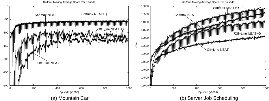
Figure 7 presents the results of combining NEAT+Q with softmax evolutionary computation, averaged over 25 runs, and compares it to using each of these methods individually, i.e. using off-line NEAT+Q (as done in Section 5.1) and using softmax evolutionary computation with regular NEAT (as done in Section 5.2). For the sake of simplicity we do not present results forε-greedy NEAT+Q though we tested it and found that it performed similarly to softmax NEAT+Q.
-300 -250 -200 -150 -100 -50 0
0 200 400 600 800 1000
Score
Episode (x1000) Uniform Moving Average Score Per Episode
-15000 -14500 -14000 -13500 -13000 -12500 -12000 -11500 -11000 -10500 -10000
0 200 400 600 800 1000
Score
Episode (x1000) Uniform Moving Average Score Per Episode
(a) Mountain Car (b) Server Job Scheduling
Off−Line NEAT
Off−Line NEAT+Q
Softmax NEAT Softmax NEAT+Q
Softmax NEAT+Q
Softmax NEAT
Off−Line NEAT
Off−Line NEAT+Q
Figure 7: The performance of combining evolutionary function approximation with on-line evolu-tionary computation compared to using each individually in the mountain car and server job scheduling domains.
In both domains, softmax NEAT+Q performs significantly better than off-line NEAT+Q. Hence, just like regular evolutionary computation, evolutionary function approximation performs better when supplemented with selection techniques traditionally used in TD methods. Surprisingly, in the mountain car domain, softmax NEAT+Q performs only as well softmax NEAT. We attribute these results to a ceiling effect, i.e. the mountain car domain is easy enough that, given an appropriate selection mechanism, NEAT is able to learn quite rapidly, even without the help of Q-learning. In the server job scheduling domain, softmax NEAT+Q does perform better than softmax NEAT, though the difference is rather modest. Hence, in both domains, the most critical factor to boosting the performance of evolutionary computation is the use of an appropriate selection mechanism.
5.4 Comparing to Previous Approaches
In the mountain car domain, the results presented above make clear that softmax NEAT+Q can rapidly learn a good policy. However, since these results use an on-line metric, performance is averaged over all members of the population. Hence, they do not reveal how close the best learned policies are to optimal. To assess this, we selected the generation champion from the final generation of each softmax NEAT+Q run and evaluated it for an additional 1,000 episodes. Then we compared this to the performance of a learner using Sarsa, a TD method similar to Q-learning (Sutton and Barto, 1998), with CMACs, a popular linear function approximator (Sutton and Barto, 1998), using a setup that matches that of Sutton (1996) as closely as possible. We found their performance to be nearly identical: softmax NEAT+Q received an average score of -52.75 while the Sarsa CMAC learner received -52.02. We believe this performance is approximately optimal, as it matches the best results published by other researchers, e.g. (Smart and Kaelbling, 2000).
This does not imply that neural networks are the function approximator of choice for the moun-tain car domain. On the contrary, Sutton’s CMACs converge in many fewer episodes. Nonetheless, these results demonstrate that evolutionary function approximation and on-line evolution make it feasible to find approximately optimal policies using neural networks, something that some previous approaches (Boyan and Moore, 1995; Pyeatt and Howe, 2001), using manually designed networks, were unable to do.
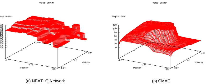
Since the mountain car domain has only two state features, it is possible to visualize the value function. Figure 8 compares the value functions learned by softmax NEAT+Q to that of Sarsa with CMACs. For clarity, the graphs plot estimated steps to the goal. Since the agent receives a reward of -1 for each timestep until reaching the goal, this is equivalent to−maxa(Q(s,a)). Surprisingly,
the two value functions bear little resemblance to one another. While they share some very general characteristics, they differ markedly in both shape and scale. Hence, these graphs highlight a fact that has been noted before (Tesauro, 1994): that TD methods can learn excellent policies even if they estimate the value function only very grossly. So long as the value function assigns the highest value to the correct action, the agent will perform well.
Value Function -1.2 -0.35 0.5 Position -0.07 0.0 0.07 Velocity 0 20 40 60 80 100 120 Steps to Goal Value Function -1.2 -0.35 0.5 Position -0.07 0.0 0.07 Velocity 100 150 200 250 300 350 400 450 500 550 600 650 Steps to Goal
(a) NEAT+Q Network (b) CMAC
In the server job scheduling domain, finding alternative approaches for comparison is less straightforward. Substantial research about job scheduling already exists but most of the methods involved are not applicable here because they do not allow jobs to be associated with arbitrary utility functions. For example, Liu and Layland (1973) present methods for job scheduling in a real-time environment, in which a hard deadline is associated with each job. McWherter et al. (2004) present methods for scheduling jobs with different priority classes. However, unlike the utility functions shown in Section 4.2, the relative importance of a job type does not change as a function of time. McGovern et al. (2002) use reinforcement learning for CPU instruction scheduling but aim only to minimize completion time.
One method that can be adapted to the server job scheduling task is the generalized cµ rule (van Mieghem, 1995), in which the server always processes at time t the oldest job of that type k which maximizes C′k(ok)/pk, where Ck′ is the derivative of the cost function for job type k, ok is the age
of the oldest job of type k and pk is the average processing time for jobs of type k. Since in our
simulation all jobs require unit time to process and the cost function is just the additive inverse of the utility function, this is equivalent to processing the oldest job of that type k that maximizes
−Uk′(ok), where Uk′ is the derivative of the utility function for job type k. The generalized cµ rule
has been proven approximately optimal given convex cost functions (van Mieghem, 1995). Since the utility functions, and hence the cost functions, are both convex and concave in our simulation, there is no theoretical guarantee about its performance in the server job scheduling domain. To see how well it performs in practice, we implemented it in our simulator and ran it for 1,000 episodes, obtaining an average score of -10,891.
Another scheduling algorithm applicable to this domain is the insertion scheduler, which per-formed the best in a previous study of a very similar domain (Whiteson and Stone, 2004). The insertion scheduler uses a simple, fast heuristic: it always selects for processing the job at the head of the queue but it keeps the queue ordered in a way it hopes will maximize aggregate utility. For any given ordering of a set of J jobs, the aggregate utility is:
∑
i∈J
Ui(ai+pi)
where Ui(·), ai, and pi are the utility function, current age, and position in the queue, respectively,
of job i. Since there are|J|! ways to order the queue, it is clearly infeasible to try them all. Instead, the insertion scheduler uses the following simple, fast heuristic: every time a new job is created, the insertion scheduler tries inserting it into each position in the queue, settling on whichever position yields the highest aggregate utility. Hence, by bootstrapping off the previous ordering, the insertion scheduler must consider only|J]orderings. We implemented the insertion scheduler in our simulator and ran it for 1,000 episodes, obtaining an average score of -13,607.
Neither the cµ rule nor the insertion scheduler perform as well as softmax NEAT+Q, whose final generation champions received an average score of -9,723 over 1,000 episodes. Softmax NEAT+Q performed better despite the fact that the alternatives rely on much greater a priori knowledge about the dynamics of the system. Both alternatives require the scheduler to have a predictive model of the system, since their calculations depend on knowledge of the utility functions and the amount of time each job takes to complete. By contrast, softmax NEAT+Q, like many reinforcement learning algorithms, assumes such information is hidden and discovers a good policy from experience, just by observing state transitions and rewards.