Knowledge-Based Kernel Approximation
Olvi L. Mangasarian [email protected]
Jude W. Shavlik [email protected]
Edward W. Wild [email protected]
Computer Sciences Department University of Wisconsin 1210 West Dayton Street Madison, WI 53706, USA
Editor: John Shawe-Taylor
Abstract
Prior knowledge, in the form of linear inequalities that need to be satisfied over multiple polyhedral sets, is incorporated into a function approximation generated by a linear combination of linear or nonlinear kernels. In addition, the approximation needs to satisfy conventional conditions such as having given exact or inexact function values at certain points. Determining such an approximation leads to a linear programming formulation. By using nonlinear kernels and mapping the prior poly-hedral knowledge in the input space to one defined by the kernels, the prior knowledge translates into nonlinear inequalities in the original input space. Through a number of computational exam-ples, including a real world breast cancer prognosis dataset, it is shown that prior knowledge can significantly improve function approximation.
Keywords: function approximation, regression, prior knowledge, support vector machines, linear
programming
1. Introduction
Support vector machines (SVMs) play a major role in classification problems (Vapnik, 2000, Cherkassky and Mulier, 1998, Mangasarian, 2000). More recently, prior knowledge has been incorporated into SVM classifiers, both to improve the classification task and to handle problems where conventional data may be few or not available (Sch¨olkopf et al., 1998, Fung et al., 2003b,a). Although SVMs have also been extensively used for regression (Drucker et al., 1997, Smola and Sch¨olkopf, 1998, Evgeniou et al., 2000, Mangasarian and Musicant, 2002), prior knowledge on properties of the func-tion to be approximated has not been incorporated into the SVM funcfunc-tion approximafunc-tion as has been done for an SVM classifier (Fung et al., 2003b,a). In this work, we introduce prior knowledge in the form of linear inequalities to be satisfied by the function on polyhedral regions of the input space for linear kernels, and on similar regions of the feature space for nonlinear kernels. These inequal-ities, unlike point-wise inequalities or general convex constraints that have already been treated in approximation theory (Mangasarian and Schumaker, 1969, 1971, Micchelli and Utreras, 1988, Deutsch, 2001), are inequalities that need to be satisfied over specific polyhedral sets. Such “prior knowledge” does not seem to have been treated in the extensive approximation theory literature.
programming formulation in that space. In Section 3 we approximate the function by a linear com-bination of nonlinear kernel functions and explicitly map the polyhedral prior knowledge in the input space to one defined by the kernel functions. This leads to a linear programming formulation in that space. In Section 4 we demonstrate the utility of our results on a number of synthetic approx-imation problems as well as a real world breast cancer prognosis dataset where we show that prior knowledge can improve the approximation. Section 5 concludes the paper with a brief summary and some possible extensions and applications of the present work.
We describe our notation now. All vectors will be column vectors unless transposed to a row vector by a prime0. The scalar (inner) product of two vectors x and y in the n-dimensional real space
Rnwill be denoted by x0y. For x∈Rn,kxk1denotes the 1-norm:
n
∑
i=1|xi|. The notation A∈Rm×nwill
signify a real m×n matrix. For such a matrix, A0will denote the transpose of A, Aiwill denote the
i-th row of A and A·jthe j-th column of A. A vector of ones in a real space of arbitrary dimension will
be denoted by e. Thus for e∈Rmand y∈Rmthe notation e0y will denote the sum of the components of y. A vector of zeros in a real space of arbitrary dimension will be denoted by 0. For A∈Rm×nand B∈Rn×k,a kernel K(A,B)maps Rm×n×Rn×kinto Rm×k. In particular, if x and y are column vectors in Rnthen, K(x0,y)is a real number, K(x0,A0)is a row vector in Rmand K(A,A0)is an m×m matrix. We shall make no assumptions on our kernels other than symmetry, that is K(x0,y)0 =K(y0,x),
and in particular we shall not assume or make use of Mercer’s positive semidefiniteness condition (Vapnik, 2000, Sch¨olkopf and Smola, 2002). The base of the natural logarithm will be denoted by ε. A frequently used kernel in nonlinear classification is the Gaussian kernel (Vapnik, 2000, Cherkassky and Mulier, 1998, Mangasarian, 2000) whose i jth element, i=1. . . ,m, j=1. . . ,k, is given by: (K(A,B))i j =ε−µkAi
0−B
·jk2, where A∈Rm×n, B∈Rn×k and µ is a positive constant.
Approximate equality is denoted by≈, while the abbreviation “s.t.” stands for “subject to”. The symbol∧denotes the logical “and” while∨denotes the logical “or”.
2. Prior Knowledge for a Linear Kernel Approximation
We begin with a linear kernel model and show how to introduce prior knowledge into such an approximation. We consider an unknown function f from Rn to R for which approximate or exact function values are given on a dataset of m points in Rn denoted by the matrix A∈Rm×n. Thus, corresponding to each point Aiwe are given an exact or inexact value of f , denoted by a real number
yi, i=1, . . . ,m. We wish to approximate f by some linear or nonlinear function of the matrix A with
unknown linear parameters. We first consider the simple linear approximation
f(x)≈w0x+b, (1)
for some unknown weight vector w∈Rn and constant b∈R which is determined by minimizing some error criterion that leads to
Aw+be−y≈0. (2)
If we consider w to be a linear combination of the rows of A, i.e. w=A0α,α∈Rm, which is similar to the dual representation in a linear support vector machine for the weight w (Mangasarian, 2000, Sch¨olkopf and Smola, 2002), we then have
This immediately suggests the much more general idea of replacing the linear kernel AA0 by some arbitrary nonlinear kernel K(A,A0): Rm×n×Rn×m−→Rm×mthat leads to the following approxima-tion, which is nonlinear in A but linear inα:
K(A,A0)α+be−y≈0. (4)
We will measure the error in (4) componentwise by a vector s∈Rmdefined by
−s≤K(A,A0)α+be−y≤s. (5)
We now drive this error down by minimizing the 1-norm of the error s together with the 1-norm ofα for complexity reduction or stabilization. This leads to the following constrained optimization prob-lem with positive parameter C that determines the relative weight of exact data fitting to complexity reduction:
min
(α,b,s) kαk1+Cksk1
s.t. −s ≤ K(A,A0)α+be−y ≤ s, (6)
which can be represented as the following linear program:
min (α,b,s,a) e
0a+Ce0s
s.t. −s ≤ K(A,A0)α+be−y ≤ s,
−a ≤ α ≤ a.
(7)
We note that the 1-norm formulation employed here leads to a linear programming formulation without regard to whether the kernel K(A,A0) is positive semidefinite or not. This would not be the case if we used a kernel-induced norm on α that would lead to a quadratic program. This quadratic program would be more difficult to solve than our linear program especially when it is nonconvex, which would be an NP-hard problem, as is the case when the kernel employed is not positive semidefinite.
We now introduce prior knowledge for a linear kernel as follows. Suppose that it is known that the function f represented by (1) satisfies the following condition. For all points x∈Rn, not necessarily in the training set but lying in the nonempty polyhedral set determined by the linear inequalities
Bx≤d, (8)
for some B∈Rk×n, the function f , and hence its linear approximation w0x+b, must dominate a given linear function h0x+β, for some user-provided(h,β)∈Rn+1. That is, for a fixed(w,b) we have the implication
Bx≤d =⇒ w0x+b≥h0x+β, (9)
or equivalently in terms ofα, where w=A0α:
Bx≤d =⇒ α0Ax+b≥h0x+β. (10)
Proposition 2.1 Prior Knowledge Equivalence. Let the set{x|Bx≤d}be nonempty. Then for a fixed(α,b,h,β), the implication (10) is equivalent to the following system of linear inequalities having a solution u∈Rk:
B0u+A0α−h=0,−d0u+b−β≥0,u≥0. (11)
Proof The implication (10) is equivalent to the following system having no solution(x,ζ)∈Rn+1: Bx−dζ≤0,(α0A−h0)x+ (b−β)ζ<0,−ζ<0. (12)
By the Motzkin theorem of the alternative (Mangasarian, 1994, Theorem 2.4.2) we have that (12) is equivalent to the following system of inequalities having a solution(u,η,τ):
B0u+ (A0α−h)η=0,−d0u+ (b−β)η−τ=0,u≥0,06= (η,τ)≥0. (13)
Ifη=0 in (13), then we contradict the nonemptiness of the knowledge set{x|Bx≤d}. Because, for x∈ {x|Bx≤d}and(u,τ)that solve (13) withη=0, we obtain the contradiction
0≥u0(Bx−d) =x0B0u−d0u=−d0u=τ>0. (14)
Henceη>0 in (13). Dividing (13) byηand redefining(u,α,τ)as(ηu,αη,ητ)we obtain (11).
Adding the constraints (11) to the linear programming formulation (7) with a linear kernel K(A,A0) =AA0, we obtain our desired linear program that incorporates the prior knowledge im-plication (10) into our approximation problem:
min (α,b,s,a,u≥0) e
0a+Ce0s
s.t. −s ≤ AA0α+be−y ≤ s,
−a ≤ α ≤ a,
A0α+B0u = h, −d0u ≥ β−b.
(15)
Note that in this linear programming formulation with a linear kernel approximation, both the approximation w0x+b=α0Ax+b to the unknown function f as well as the prior knowledge are linear in the input data A of the problem. This is somewhat restrictive, and therefore we turn now to our principal concern in this work, which is the incorporation of prior knowledge into a nonlinear kernel approximation.
3. Knowledge-Based Nonlinear Kernel Approximation
In this part of the paper we will incorporate prior knowledge by using a nonlinear kernel in both the linear programming formulation (7) as well as in the prior knowledge implication (10). We begin with the latter, the linear prior knowledge implication (10). If we again consider x as a linear combination of the rows of A, that is
x=A0t, (16)
then the implication (10) becomes
for a given fixed (α,b). The assumption (16) is not restrictive for the many problems where a sufficiently large number of training data points are available so that any vector in input space can be represented as a linear combination of the training data points.
If we now ”kernelize” the various matrix products in the above implication, we have the impli-cation
K(B,A0)t≤d =⇒ α0K(A,A0)t+b≥h0A0t+β. (18)
We note that the two kernels appearing in (18) need not be the same and neither needs to satisfy Mercer’s positive semidefiniteness condition. In particular, the first kernel of (18) could be a linear kernel which renders the left side of the implication of (18) the same as that of (17). We note that for a nonlinear kernel, implication (18) is nonlinear in the input space data, but is linear in the implication variable t. We have thus mapped the polyhedral implication (9) into a nonlinear one (18) in the input space data. Assuming for simplicity that the kernel K is symmetric, that is K(B,A0)0=K(A,B0), it follows directly by Proposition 2.1 that the following equivalence relation
holds for implication (18).
Proposition 3.1 Nonlinear Kernel Prior Knowledge Equivalence. Let the set
{t|K(B,A0)t≤d}be nonempty. Then for a given(α,b,h,β), the implication (18) is equivalent to the following system of linear inequalities having a solution u∈Rk:
K(A,B0)u+K(A,A0)α−Ah=0,−d0u+b−β≥0,u≥0. (19)
We now append the constraints (19), which are equivalent to the nonlinear kernel implication (18), to the linear programming formulation (7). This gives the following linear program for approximating a given function with prior knowledge using a nonlinear kernel:
min (α,b,s,a,u≥0) e
0a+Ce0s
s.t. −s ≤ K(A,A0)α+be−y ≤ s,
−a ≤ α ≤ a,
K(A,B0)u+K(A,A0)α = Ah,
−d0u ≥ β−b.
(20)
Since we are not certain that the prior knowledge implication (18) is satisfiable, and since we wish to balance the influence of prior knowledge with that of fitting conventional data points, we need to introduce error variables z andζassociated with the last two constraints of the linear program (20). These error variables are then driven down by a modified objective function as follows:
min (α,b,s,a,z,(u,ζ)≥0) e
0a+Ce0s+µ
1e0z+µ2ζ
s.t. −s ≤ K(A,A0)α+be−y ≤ s,
−a ≤ α ≤ a,
−z ≤ K(A,B0)u+K(A,A0)α−Ah ≤ z,
−d0u+ζ ≥ β−b,
(21)
data versus the given prior knowledge. One way to choose these parameters is to set aside a “tuning set” of data points and then choose the parameters so as to give a best fit of the tuning set. We also note that all three kernels appearing in (21) could possibly be distinct kernels from each other and none needs to be positive semidefinite. In fact, the kernel K(A,B0)could be the linear kernel AB0 which was was actually tried in some of our numerical experiments without a noticeable change from using a Gaussian kernel.
We now turn to our numerical experiments.
4. Numerical Experiments
The focus of this paper is mainly theoretical. However, in order to illustrate the power of the proposed formulation, we tested our algorithm on three synthetic examples and one real world example with and without prior knowledge. Two of the synthetic examples are based on the “sinc” function which has been extensively used for kernel approximation testing (Vapnik et al., 1997, Baudat and Anouar, 2001), while the third synthetic example is a two-dimensional hyperboloid. All our results indicate significant improvement due to prior knowledge. The parameters for the synthetic examples were selected using a combination of exhaustive search and a simple variation on the Nelder-Mead simplex algorithm (Nelder and Mead, 1965) that uses only reflection, with average error as the criterion. The chosen parameter values are given in the captions of relevant figures.
4.1 One-Dimensional Sinc Function
We consider the one-dimensional sinc function
f(x) =sinc(x) =sinπx
πx . (22)
−3 −2 −1 0 1 2 3 −1.5
−1 −0.5 0 0.5 1
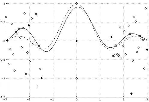
Figure 1: The one-dimensional sinc function sinc(x) = sinπxπx (dashed curve) and its Gaussian kernel approximation without prior knowledge based on the 55 points shown by diamonds. The nine solid diamonds depict the “support” points used by the nonlinear Gaussian kernel in generating the approximation of sinc(x). That is, they are the rows Ai of A for which
αi 6=0 in the solution of the nonlinear Gaussian kernel approximation of (7) for f(x):
f(x)≈K(x0,A0)α+b. The approximation has an average error of 0.3113 over a grid of 100 points in the interval[−3,3]. Parameter values used: µ=7,C=5.
−3 −2 −1 0 1 2 3 −1.5
−1 −0.5 0 0.5 1
Figure 2: The one-dimensional sinc function sinc(x) = sinπx
πx (dashed curve) and its Gaussian
ker-nel approximation with prior knowledge based on 55 points, shown by diamonds, which are the same as those of Figure 1. The seven solid diamonds depict the “support” points used by the nonlinear Gaussian kernel in generating the approximation of sinc(x). The prior knowledge consists of the implication −14 ≤x≤ 14 ⇒ f(x)≥ sinπ/(π/44), which is implemented by replacing f(x) by its nonlinear kernel approximation (23). The ap-proximation has an average error of 0.0901 over a grid of 100 points in the interval
−3 −2 −1 0 1 2 3 −3 −2 −1 0 1 2 3 −0.4 −0.2 0 0.2 0.4 0.6 0.8 1
Figure 3: The exact product sinc function f(x1,x2) =sinπx1πx1sinπx2πx2.
−3 −2 −1 0 1 2 3 −3 −2 −1 0 1 2 3 −0.4 −0.2 0 0.2 0.4 0.6 0.8 1
Figure 4: Gaussian kernel approximation of the product sinc function f(x1,x2) =sinπx1πx1sinπx2πx2 based on 211 exact function values plus 2 incorrect function values, but without prior knowl-edge. The approximation has an average error of 0.0501 over a grid of 2500 points in the set{[−3,3]×[−3,3]}. Parameter values used: µ=0.2,C=106.
−3 −2 −1 0 1 2 3 −3 −2 −1 0 1 2 3 −0.4 −0.2 0 0.2 0.4 0.6 0.8 1
Figure 5: Gaussian kernel approximation of the product sinc function based on the same 213 function values as Figure 4 plus prior knowledge consisting of(x1,x2)∈ {[−0.1,0.1]×
actual limit of the sinc function at 0. The other values at x=0 are 0 and−1 which are intended to be misleading to the approximation.
Figure 1 depicts sinc(x)by a dashed curve and its approximation without prior knowledge by a solid curve based on the 55 points shown by diamonds. The nine solid diamonds depict “sup-port” points, that is rows Ai of A for whichαi6=0 in the solution of the nonlinear Gaussian kernel
approximation of (7) for f(x):
f(x)≈K(x0,A0)α+b. (23)
The approximation in Figure 1 has an average error of 0.3113. This error is computed by averaging over a grid of 100 equally spaced points in the interval[−3,3].
Figure 2 depicts sinc(x)by a dashed curve and its much better approximation with prior knowl-edge by a solid curve based on the 55 points shown, which are the same as those of Figure 1. The seven solid diamond points are “support” points, that is rows Ai of A for which αi 6=0 in
the solution of the nonlinear Gaussian kernel approximation (23) of (21) for f(x). The approx-imation in Figure 2 has an average error of 0.0901 computed over a grid of 100 equally spaced points on [−3,3]. The prior knowledge used to approximate the one-dimensional sinc function is −1
4 ≤x≤ 1
4 ⇒ f(x)≥
sin(π/4)
π/4 . The value
sin(π/4)
π/4 is the minimum of sinc(x) on the knowledge interval[−14,14]. This prior knowledge is implemented by replacing f(x) by its nonlinear kernel approximation (23) and then using the implication (18) as follows:
K(I,A0)t≤1
4 ∧ K(−I,A
0)t≤ 1
4=⇒α
0K(A,A0)t+b≥sin(π/4)
π/4 . (24)
4.2 Two-Dimensional Sinc Function
Our second example is the two-dimensional sinc(x)function for x∈R2:
f(x1,x2) =sinc(x1)sinc(x2) = sinπx1
πx1
sinπx2
πx2
. (25)
The given data for the two-dimensional sinc function includes 210 points in the region{(x1,x2)|(−3≤ x1≤ −1.4303∨1.4303≤x1≤3)∧(−3≤x2≤ −1∨1≤x2≤3)}. This region excludes the largest bump in the function centered at(x1,x2) = (0,0). The given values are exact function values. There are also three values given at(x1,x2) = (0,0), similar to the previous example with the one dimen-sional sinc. The first value is the actual limit of the function at(0,0), which is 1. The other two values are 0 and−1. These last two values are intended to mislead the approximation.
Figure 3 depicts the two-dimensional sinc function of (25). Figure 4 depicts an approximation of sinc(x1)sinc(x2)without prior knowledge by a surface based on the 213 points described above. The approximation in Figure 4 has an average error of 0.0501. This value is computed by averaging over a grid of 2500 equally spaced points in{[−3,3]×[−3,3]}.
−5
0
5 −5
0 5
−25 −20 −15 −10 −5 0 5 10 15 20 25
Figure 6: The exact hyperboloid function f(x1,x2) =x1x2.
−5
0
5 −5
0 5
−25 −20 −15 −10 −5 0 5 10 15 20 25
Figure 7: Gaussian kernel approximation of the hyperboloid function f(x1,x2) =x1x2based on 11 exact function values along the line x2=x1,x1 ∈ {−5,−4, . . . ,4,5}, but without prior knowledge. The approximation has an average error of 4.8351 over 2500 points in the set {[−5,5]×[−5,5]}. Parameter values used: µ=0.361,C=145110.
−5 0
5 −5
0 5
−25 −20 −15 −10 −5 0 5 10 15 20 25
{[−3,3]×[−3,3]}. The prior knowledge consists of the implication
(x1,x2)∈ {[−0.1,0.1]×[−0.1,0.1]} ⇒ f(x1,x2)≥(
sin(π/10)
π/10 ) 2.
The value (sinπ/(π/1010))2 is equal to the minimum value of sinc(x
1)sinc(x2) on the knowledge set {[−0.1,0.1]×[−0.1,0.1]}. This prior knowledge is implemented by replacing f(x1,x2)by its non-linear kernel approximation (23) and then using the implication (18).
4.3 Two-Dimensional Hyperboloid Function
Our third example is the two-dimensional hyperboloid function
f(x1,x2) =x1x2. (26) For the two-dimensional hyperboloid function, the given data consists of 11 points along the line x2=x1,x1∈ {−5,−4, . . . ,4,5}. The given values at these points are the actual function values. Figure 6 depicts the two-dimensional hyperboloid function of (26). Figure 7 depicts an approx-imation of the hyperboloid function, without prior knowledge, by a surface based on the 11 points described above. The approximation in Figure 7 has an average error of 4.8351 computed over a grid of 2500 equally spaced points in{[−5,5]×[−5,5]}.
Figure 8 depicts a much better approximation of the hyperboloid function by a nonlinear surface based on the same 11 points above plus prior knowledge. The approximation in Figure 8 has an average error of 0.2023 computed over a grid of 2500 equally spaced points in{[−5,5]×[−5,5]}. The prior knowledge consists of the following two implications:
(x1,x2)∈ {(x1,x2)|− 1
3x1≤x2≤ − 2
3x1} ⇒ f(x1,x2)≤10x1 (27)
and
(x1,x2)∈ {(x1,x2)|− 2
3x1≤x2≤ − 1
3x1} ⇒ f(x1,x2)≤10x2. (28)
These implications are implemented by replacing f(x1,x2) by its nonlinear kernel approximation (23) and then using the implication (18). The regions on which the knowledge is given are cones on which x1x2 is negative. Since the two implications are analogous, we explain (27) only. This implication is justified on the basis that x1x2≤10x1over the knowledge cone{(x1,x2)|−13x1≤x2≤ −23x1}for sufficiently large x2, that is x2≥10. This is intended to capture coarsely the global shape of f(x1,x2)and succeeds in generating a more accurate overall approximation of the function. 4.4 Predicting Lymph Node Metastasis
lymph nodes as a function of thirty available cytological features and one histological feature. The cytological features are obtained from a fine needle aspirate during the diagnostic procedure while the histological feature is obtained during surgery. Our proposed knowledge-based approximation can be used to improve the determination of such a function, f : R31−→R, that predicts the num-ber of metastasized lymph nodes. For example, in certain polyhedral regions of R31, past training data indicate the existence of a substantial number of metastasized lymph nodes, whereas certain other regions indicate the unlikely presence of any metastasis. This knowledge can be applied to obtain a hopefully more accurate lymph node function f than that based on numerical function approximation alone.
We have performed preliminary experiments with the Wisconsin Prognostic Breast Cancer (WPBC) data available from (Murphy and Aha, 1992). In our experiments we reduced R31to R4 and predicted the number of metastasized lymph nodes based on three cytological features: mean cell texture, worst cell smoothness, and worst cell area, as well as the histological feature tumor size. The tumor size is an obvious histological feature to include, while the three other cytological features were the same as those selected for breast cancer diagnosis in (Mangasarian, 2001). Thus, we are approximating a function f : R4−→R. Note that the online version of the WPBC data con-tains four entries with no lymph node information which were removed for our experiments. After removing these entries, we were left with 194 examples in our dataset.
To simulate the procedure of an expert obtaining prior knowledge from past data we used the following procedure. First we took a random 20% of the dataset to analyze as “past data”. Inspecting this past data, we choose the following background knowledge:
x1≥22.4 ∧ x2≥0.1 ∧ x3≥1458.9 ∧ x4≥3.1 =⇒ f(x1,x2,x3,x4)≥1, (29) where x1,x2,x3,and x4denote mean texture, worst smoothness, worst area, and tumor size respec-tively. This prior knowledge is based on a typical oncological surgeon’s advice that larger values of the variables are likely to result in more metastasized lymph nodes. The constants in (29) were chosen by taking the average values of x1, . . . ,x4 for the entries in the past data with at least one metastasized lymph node.
We used ten-fold cross validation to compare the average absolute error between an approxima-tion without prior knowledge and an approximaapproxima-tion with the prior knowledge of Equaapproxima-tion (29) on the 80% of the data that was not used as “past data” to generate the constants in (29). Parameters in (21) using a Gaussian kernel were chosen using the Nelder-Mead algorithm on a tuning set taken from the training data for each fold. The average absolute error of the function approximation with no prior knowledge was 3.75 while the average absolute error with prior knowledge was 3.35, a 10.5% reduction. The mean function value of the data used in the ten-fold cross validation exper-iments is 3.30, so neither approximation is accurate. However, these results indicate that adding prior knowledge does indeed improve the function approximation substantially. Hopefully more sophisticated prior knowledge, based on a more detailed analysis of the data and consultation with domain experts, will further reduce the error.
holding the ball and attempting a pass to a teammate. It has been demonstrated that providing prior knowledge can improve the choice of actions significantly (Kuhlmann et al., 2004, Maclin and Shavlik, 1996). One example of advice (that is, prior knowledge) that has been successfully used in this domain is the simple advice that “if no opponent is within 8 meters, holding the ball is a good idea.” In our approach we approximate a value function v as a function of states and actions. Advice can be stated as the following implication, assuming two opponents:
d1≥8 ∧ d2≥8 ∧ a=h =⇒ v≥c, (30) where d1 denotes the distance to Opponent 1, d2 the distance to Opponent 2, a=h the action of holding the ball, v the predicted value, and c is some constant. It is hoped that this “advice” can help in generating an improved value function v based on the current description of the state of the soccer game.
5. Conclusion and Outlook
We have presented a knowledge-based formulation of a nonlinear kernel SVM approximation. The approximation is obtained using a linear programming formulation with any nonlinear symmetric kernel and with no positive semidefiniteness (Mercer) condition assumed. The issues associated with sampling the knowledge sets in order to generate function values (that is, a matrix A and a corresponding vector y) in situations where there are no conventional data points constitute an interesting topic for future research. Additional future work includes refinement of prior knowledge and applications to medical problems, computer vision, microarray gene classification, and efficacy of drug treatment, all of which have prior knowledge available.
Acknowledgments
We are grateful to our colleagues Rich Maclin and Dave Musicant for constructive comments. Re-search described in this UW Data Mining Institute Report 03-05, October 2003, was supported by NSF Grants CCR-0138308, and IRI-9502990, by NLM Grant 1 R01 LM07050-01, by DARPA ISTO Grant HR0011-04-0007, by PHS Grant 5 T15 LM07359-02 and by Microsoft.
References
G. Baudat and F. Anouar. Kernel-based methods and function approximation. In International Joint Conference on Neural Networks, pages 1244–1249, Washington, D.C., 2001.
V. Cherkassky and F. Mulier. Learning from Data - Concepts, Theory and Methods. John Wiley & Sons, New York, 1998.
F. Deutsch. Best Approximation in Inner Product Spaces. Springer-Verlag, Berlin, 2001.
T. Evgeniou, M. Pontil, and T. Poggio. Regularization networks and support vector machines. In A. Smola, P. Bartlett, B. Sch¨olkopf, and D. Schuurmans, editors, Advances in Large Margin Classifiers, pages 171–203, Cambridge, MA, 2000. MIT Press.
G. Fung, O. L. Mangasarian, and J. Shavlik. Knowledge-based nonlinear kernel classifiers. Tech-nical Report 03-02, Data Mining Institute, Computer Sciences Department, University of Wis-consin, Madison, WisWis-consin, March 2003a. ftp://ftp.cs.wisc.edu/pub/dmi/tech-reports/02-03.ps. Conference on Learning Theory (COLT 03) and Workshop on Kernel Machines, Washington D.C., August 24-27, 2003. Proceedings edited by M. Warmuth and B. Sch¨olkopf, Springer Ver-lag, Berlin, 2003, 102-113.
G. Fung, O. L. Mangasarian, and J. Shavlik. Knowledge-based support vector machine classifiers. In Suzanna Becker, Sebastian Thrun, and Klaus Obermayer, editors, Advances in Neural Infor-mation Processing Systems 15, pages 521–528. MIT Press, Cambridge, MA, October 2003b. ftp://ftp.cs.wisc.edu/pub/dmi/tech-reports/01-09.ps.
G. Kuhlmann, P. Stone, R. Mooney, and J. Shavlik. Guiding a reinforcement learner with natural language advice: Initial results in robocup soccer. In Proceedings of the AAAI Workshop on Supervisory Control of Learning and Adaptive Systems, San Jose, CA, 2004.
Y.-J. Lee, O. L. Mangasarian, and W. H. Wolberg. Survival-time classification of breast cancer pa-tients. Technical Report 01-03, Data Mining Institute, Computer Sciences Department, University of Wisconsin, Madison, Wisconsin, March 2001. ftp://ftp.cs.wisc.edu/pub/dmi/tech-reports/01-03.ps. Computational Optimization and Applications 25, 2003, 151-166.
R. Maclin and J. Shavlik. Creating advice-taking reinforcement learners. Machine Learning, 22, 1996.
O. L. Mangasarian. Nonlinear Programming. SIAM, Philadelphia, PA, 1994.
O. L. Mangasarian. Generalized support vector machines. In A. Smola, P. Bartlett, B. Sch¨olkopf, and D. Schuurmans, editors, Advances in Large Margin Classifiers, pages 135–146, Cambridge, MA, 2000. MIT Press. ftp://ftp.cs.wisc.edu/math-prog/tech-reports/98-14.ps.
O. L. Mangasarian. Data mining via support vector machines, July 23-27, 2001.
http://ftp.cs.wisc.edu/math-prog/talks/ifip3tt.ppt.
O. L. Mangasarian and D. R. Musicant. Large scale kernel regression via linear programming. Machine Learning, 46:255–269, 2002. ftp://ftp.cs.wisc.edu/pub/dmi/tech-reports/99-02.ps.
O. L. Mangasarian and L. L. Schumaker. Splines via optimal control. In I. J. Schoenberg, editor, Approximations with Special Emphasis on Splines, pages 119–156, New York, 1969. Academic Press.
O. L. Mangasarian and L. L. Schumaker. Discrete splines via mathematical programming. SIAM Journal on Control, 9:174–183, May 1971.
C. A. Micchelli and F. I. Utreras. Smoothing and interpolation in a convex subset of a hilbert space. SIAM Journal of Statistical Computing, 9:728–746, 1988.
P. M. Murphy and D. W. Aha. UCI machine learning repository, 1992.
www.ics.uci.edu/∼mlearn/MLRepository.html.
J. A. Nelder and R. Mead. A simplex method for function minimization. The Computer Journal, 7: 308–313, 1965.
B. Sch¨olkopf, P. Simard, A. Smola, and V. Vapnik. Prior knowledge in support vector kernels. In M. Jordan, M. Kearns, and S. Solla, editors, Advances in Neural Information Processing Systems 10, pages 640 – 646, Cambridge, MA, 1998. MIT Press.
B. Sch¨olkopf and A. Smola. Learning with Kernels. MIT Press, Cambridge, MA, 2002.
A. Smola and B. Sch¨olkopf. On a kernel-based method for pattern recognition, regression, approx-imation and operator inversion. Algorithmica, 22:211–231, 1998.
P. Stone and R. Sutton. Scaling reinforcement learning toward robocup soccer. In Proceedings of the Eighteenth International Conference on Machine Learning (ICML’01), Williams, MA, 2001.
R. Sutton and A. Barto. Reinforcement Learning: An Introduction. MIT Press, Cambridge, MA, 1998.
V. N. Vapnik. The Nature of Statistical Learning Theory. Springer, New York, second edition, 2000.
V. N. Vapnik, S. E. Golowich, and A. Smola. Support vector method for function approximation, regression estimation and signal processing. In Neural Information Processing Systems Volume 9, pages 281–287, Cambridge, MA, 1997. MIT Press.