Some Dichotomy Theorems for Neural Learning Problems

Some Dichotomy Theorems for Neural Learning Problems

Michael Schmitt [email protected]

Lehrstuhl Mathematik und Informatik Fakult¨at f¨ur Mathematik

Ruhr-Universit¨at Bochum D–44780 Bochum, Germany

Editor: Manfred K. Warmuth

Abstract

The computational complexity of learning from binary examples is investigated for linear threshold neurons. We introduce combinatorial measures that create classes of infinitely many learning prob-lems with sample restrictions. We analyze how the complexity of these probprob-lems depends on the values for the measures. The results are established as dichotomy theorems showing that each prob-lem is either NP-complete or solvable in polynomial time. In particular, we consider consistency and maximum consistency problems for neurons with binary weights, and maximum consistency problems for neurons with arbitrary weights. We determine for each problem class the dividing line between the NP-complete and polynomial-time solvable problems. Moreover, all efficiently solvable problems are shown to have constructive algorithms that require no more than linear time on a random access machine model. Similar dichotomies are exhibited for neurons with bounded threshold. The results demonstrate on the one hand that the consideration of sample constraints can lead to the discovery of new efficient algorithms for non-trivial learning problems. On the other hand, hard learning problems may remain intractable even for severely restricted samples.

Keywords: linear threshold neuron, consistency problem, computational complexity, linear-time

algorithm, NP-completeness

1. Introduction

The ability to learn is certainly one of the most challenging qualities that people have ever demanded from computers. There is no doubt that a major advancement in the development of learning algo-rithms has been made due to the use of neural networks. Today, they provide the basis for some of the most successful learning techniques. This achievement, however, is compromised by the fact that the running times required by neural learning algorithms are often immense. On the theoretical side, investigations of the computational complexity of learning problems have supported the con-jecture that neural learning is generally hard: Theory considers an algorithm as efficient if its run-ning time is bounded by a polynomial in the input length. Based on the theory of NP-completeness (see, e.g., Garey and Johnson, 1979) researchers have established numerous intractability results for neural learning problems. Consequently, no efficient, that is, polynomial-time, algorithm for solving these problems can exist if the complexity classes P and NP are different. (See, e.g., ˇS´ıma, 2002, for a comprehensive list of hardness results concerning single neurons and neural networks.)

sample, there is some hypothesis in the class that is consistent with all examples, that is, assigns the correct output values. The consistency problem is also known as loading problem (Judd, 1990), fitting problem (Natarajan, 1991), or training problem (Blum and Rivest, 1992). A variant of the consistency problem is the maximum consistency problem, also known as minimizing disagreement problem. Its instances consist of a training sample and a natural number k. The question is to decide whether there is a hypothesis consistent with some subset of at least k examples. The maximum consistency problem is a generalization of the consistency problem in that the latter is a subproblem of the former: The consistency problem can be obtained from the maximum consistency problem by setting k equal to the number of examples. Consequently, if for a given hypothesis class the consistency problem is NP-hard then the maximum consistency problem is NP-hard, too. Consis-tency and maximum consisConsis-tency problems are studied as key problems in the computational models of learning known as probably approximately correct (PAC) learning and agnostic PAC learning. A fundamental result states that, under the assumption that the complexity classes RP and NP are different, PAC learning cannot be efficient for a hypothesis class if the consistency problem for this class is NP-hard (Pitt and Valiant, 1988; Blumer et al., 1989). An analogous result links the model of agnostic PAC learning with the maximum consistency problem (Kearns et al., 1994; Anthony and Bartlett, 1999).

There has been perseverating interest in theoretical issues of learning using single neurons as hypothesis class (see, e.g., Servedio, 2002, and the references there). One of the extensively studied models is the linear threshold neuron, also known as McCulloch-Pitts neuron (McCulloch and Pitts, 1943). It serves as elementary building block for many neural network types (see, e.g., Haykin, 1999). While the linear threshold neuron has arbitrary real-valued weights, a variant that has gained particular attention is obtained by restricting the weights to binary values (see, e.g., Golea and Marchand, 1993; Fang and Venkatesh, 1996; Kim and Roche, 1998; Sommer and Palm, 1999). With binary weights a linear threshold neuron is still able to compute fundamental Boolean functions such as conjunction, disjunction, and r-of-k threshold functions1that have been of specific interest in questions of learning (Hampson and Volper, 1986; Littlestone, 1988; Pitt and Valiant, 1988).

In this article, we investigate the complexity of consistency and maximum consistency prob-lems for linear threshold neurons with binary and with arbitrary weights. We do this under the assumption that the training examples are binary, that is, have entries from{0,1}. While the con-sistency problem for linear threshold neurons with arbitrary weights is known to be solvable in polynomial time using methods of linear programming (see, e.g., Maass and Tur ´an, 1994; Anthony and Bartlett, 1999) we focus on those problems that are NP-complete: The consistency problem for linear threshold neurons with binary weights has been proved to be NP-complete by Pitt and Valiant (1988). Hence, also the maximum consistency problem for these neurons is NP-complete. The maximum consistency problem for linear threshold neurons with arbitrary weights is known to be NP-complete from the work of H ¨offgen et al. (1995) improving an earlier result by Amaldi (1991). We take a closer look at these problems by introducing and analyzing subproblems. In other words, we raise the question whether these problems become easier when the training samples are restricted. To this end we define two combinatorial measures for characterizing the complexity of a sample. The first quantity, called coincidence, indicates the maximum number of components in which any two examples are both non-zero. The second measure, called sparseness, represents the maximum number of non-zero components, or the Hamming-weight, of any example. The

choice of these measures is guided by the insight that learning for single neurons is easy when the coincidence or the sparseness of the samples is severely limited. So, it is not hard to see that the consistency problem is trivial when the examples are pairwise orthogonal, that is, when the sample has coincidence zero. The same observation can be made for the case when the examples are required to be extremely sparse. A further motivation for introducing sparseness arises from investigations of neural associative memories. In these, sparseness has been shown to be relevant for their storage capacities using specific learning rules (Palm, 1980).

By introducing coincidence and sparseness as sample restrictions we obtain infinite classes of consistency and maximum consistency problems: For each pair c,d of natural numbers there is the (maximum) consistency problem with coincidence c and sparseness d. The question arises how the complexity of the consistency and the maximum consistency problems depends on the values for coincidence and sparseness. As one of the main results it emerges that these problems are already NP-complete when coincidence and sparseness are bounded, a fact that does not follow from previous work. Moreover, we give a complete categorization of these consistency and maximum consistency problems into NP-complete and polynomial-time solvable. In other words, we establish so-called dichotomy theorems for these problems. Given an infinite class of problems, a dichotomy theorem states that each problem is either NP-complete or contained in the complexity class P. Thus, if P6=NP, the dichotomy theorem separates the efficiently solvable problems from the intractable ones. A dichotomy theorem is an important finding since it is known that if P and NP are different then there are infinitely many problems in NP that are neither in P nor NP-complete (see, e.g., Garey and Johnson, 1979). It is therefore significant that none of these problems of intermediate complexity is found among the (maximum) consistency problems considered here. In computational complexity there are only a few dichotomy theorems known. The most popular one is that for k-SAT which states that the satisfiability problem for conjunctions of Boolean clauses, where each clause has size at most k, is NP-complete when k is at least 3 and solvable in polynomial time for k at most 2. The dichotomy of k-SAT emerges as a special case of the renowned result of Schaefer (1978) who established a more general dichotomy theorem for satisfiability problems. Concerning more recent results we refer to Kirousis and Kolaitis (2003) where also a brief survey on dichotomy theorems in computational complexity is given. The first dichotomy theorem in conjunction with learning problems has been provided by Dalmau (1999) for learning quantified Boolean formulas (see also Dalmau and Jeavons, 2003).

in linear time on a RAM. For the maximum consistency problem and linear threshold neurons with binary weights NP-completeness is found at a value for the threshold of 1 or greater, whereas linear-time solvability holds when the threshold is equal to 0.

The dichotomy theorems presented here extend the NP-completeness results for learning with single neurons to an infinite class of subproblems. Therefore, they confirm that neural learning belongs to the hardest computational problems that one needs to solve in practice. On the other hand, those problems that we find to be solvable in polynomial time can be solved even in linear time on a RAM. The algorithms designed for these problems give interesting new insights. Moreover, efficiently solvable subproblems have been successfully used for the design of improved heuristics for NP-complete problems (Zheng and Stuckey, 2002). Therefore, it is reasonable to expect that the new linear-time algorithms presented here may lead to new and faster heuristics for learning in single neurons and neural networks.

In Section 2 we introduce the definitions of the basic concepts. The dichotomy theorems are stated in Section 3. The proofs are given in the following two sections: Section 4 is concerned with the NP-completeness results while the linear-time algorithms are presented in Section 5. Section 6 is devoted to some conclusions and open questions. In the appendix we establish the NP-completeness of a new variant of the satisfiability problem that is used in Section 4. We assume that the reader is familiar with the theory of NP-completeness as covered, for instance, by Garey and Johnson (1979).

Bibliographic Note. Some of the results in this article have been previously described in a

technical report (Schmitt, 1994a) and presented at the International Conference on Artificial Neural Networks, ICANN ’95, in Paris (Schmitt, 1995). This article is a thoroughly revised and extended version of these papers.

2. Neurons, Samples, Problems, and Algorithms

We begin by defining the neuron model and the function classes associated with it. Then we in-troduce the notion of a sample and specify the computational problems involved with neurons and samples. Finally, with regard to the linear-time algorithms presented in Section 5, we describe the computer model of the random access machine (RAM) on which the time bounds rely.

2.1 Neurons

A linear threshold neuron has parameters w1, . . . ,wn,t∈R, where w1, . . . ,wn are the weights and t is the threshold. The class of linearly separable Boolean functions in n variables, denoted

Ln

, is the class of functions f :{0,1}n _{→ {0,1} that can be computed by a linear threshold neuron.} Specifically, for every f ∈

Ln

there are weights w1, . . . ,wn and a threshold t such that for all x∈

{0,1}n_,

f(x) =

1 if w1x1+· · ·+wnxn≥t, 0 otherwise.

We use

Bn

to denote the subclass of linearly separable Boolean functions in n variables that can be computed by a linear threshold neuron using only binary weights, that is, w1, . . . ,wn∈ {0,1}. Further,

B

_n`is the subclass of functions in

Bn

that can be computed with threshold t ≤`. Clearly, a value of`∈ {0, . . . ,n}is sufficient and we have

B

n

n =

Bn

.

By omitting the subscript n we refer to the union of the respective classes such as, for instance,

L

=S

2.2 Samples

A sample S is a finite set S⊆ {0,1}n_{× {0,1}. The elements of S are called examples. Given a} sample S, the set of positive examples Pos(S) and the set of negative examples Neg(S) of S are defined by

Pos(S) = {x|(x,1)∈S},

Neg(S) = {x|(x,0)∈S}.

A sample may contain examples that are both positive and negative. Otherwise, that is, if Pos(S)∩

Neg(S) =/0, the sample is said to be consistent.2The domain of a sample S, denoted Dom(S), is the set

Dom(S) = Pos(S)∪Neg(S).

We introduce two combinatorial measures that assign natural numbers to samples: coincidence and sparseness. The coincidence of a sample S, denoted Coin(S), is

Coin(S) =

max{x·y|x,y∈Dom(S),x6=y} if|S| ≥2,

0 otherwise,

where x·y denotes the inner product. The sparseness of S, Sparse(S), is

Sparse(S) =

max{x·x|x∈Dom(S)} if S6=/0,

0 otherwise.

Thus, Coin(S)is the maximum number of components in which two different elements in the do-main of S have a 1 in common, and Sparse(S) is the maximum number of 1s, or the Hamming weight, of an element. Note that Coin(S)≤Sparse(S). Thus, bounding the sparseness of samples by some constant also bounds their coincidence by the same constant.

2.3 Consistency Problems

Given a sample S, a function f is said to be consistent with S if f satisfies f(x) =a for all(x,a)∈S. The consistency problem for a class

F

of Boolean functions is the problem to decide whether for an input sample S there exists some function f ∈

F

that is consistent with S. Loading problem, fitting problem, and training problem are synonyms for the consistency problem.

Let

F

be a class of Boolean functions and let c,d∈N_{. We define the following consistency}

problems for

F

with sample restrictions:

F

-CONSISTENCY WITHCOINCIDENCEc Instance: A sample S with Coin(S)≤c.

Question: Is there a function f ∈

F

that is consistent with S?

F

-CONSISTENCY WITHSPARSENESSd Instance: A sample S with Sparse(S)≤d.

Question: Is there a function f ∈

F

that is consistent with S?

The definition of the problem

F

-CONSISTENCY WITH COINCIDENCE c AND SPARSENESS d is similar.

The instances of the maximum consistency problem for a class

F

of functions consist of a sample S and a number k∈N_{. The question is whether there exists a subset of S with at least k}

elements and a function f ∈

F

consistent with that subset. Given numbers c,d∈N_{, we define}

maximum consistency problems for

F

with sample restrictions as follows:

MAX-F-CONSISTENCY WITHCOINCIDENCEc

Instance: A sample S with Coin(S)≤c and a natural number k.

Question: Is there a subsample S0⊆S with|S0| ≥k and a function f ∈

F

that is consistent with S0?

MAX-

F

-CONSISTENCY WITHSPARSENESSd

Instance: A sample S with Sparse(S)≤d and a natural number k.

Question: Is there a subsample S0⊆S with|S0| ≥k and a function f ∈

F

that is consistent with S0?

Further, we consider the problem called MAX-F-CONSISTENCY WITH COINCIDENCE c AND SPARSENESSd, which is the problem where the instances satisfy both constraints.

There are some natural relationships among the complexities of these problems. Clearly, an algorithm that solves the consistency problem with sparseness d solves also every consistency lem with sparseness less than d for the same function class. Furthermore, if the consistency prob-lem is shown to be NP-hard for some sparseness d then it follows that all consistency probprob-lems with sparseness larger than d for the same function class are NP-hard as well, since the reduction established for sparseness d is also valid for larger bounds on the sparseness.

Similar considerations can be made with regard to coincidence. Moreover, complexity results for consistency problems with bounded coincidence have consequences for the complexity of con-sistency problems with bounded sparseness, and vice versa. In particular, an algorithm that solves the consistency problem for coincidence c solves also the consistency problem for sparseness c+1 since every sample with sparseness at most c+1 has coincidence no more than c. (Note that coin-cidence is measured using non-identical pairs only.) Correspondingly, NP-hardness for sparseness d implies NP-hardness for coincidence d−1.

Analogous interdependences hold among the maximum consistency problems with sample re-strictions. Additionally, maximum consistency problems are related to consistency problems in that the consistency problem is a subproblem of the corresponding maximum consistency problem. The former is obtained from the latter by letting the number k be equal to the cardinality of the sample.

2.4 Linear-Time Algorithms

subtraction, whereas multiplication and division are not available. We give time bounds for RAMs in the uniform measure, that is, the execution of an instruction counts as one unit of time. It is known that every RAM that requires time t(n) in the uniform measure can be simulated on a multi-tape Turing machine in time O(t3(n))(Cook and Reckhow, 1973). In particular, a linear-time algorithm on a RAM ensures that the problem it solves belongs to P.

3. Dichotomy Theorems

We present five dichotomy theorems about the complexity of consistency problems with sample restrictions. They deal with the function classes

B

,

B

`, and

L

introduced in Section 2.1 and the consistency problems and maximum consistency problems with sample restrictions defined in Sec-tion 2.3. The dichotomy theorems establish that, with one excepSec-tion, each of these problems is either NP-complete or solvable in polynomial time. The latter is shown by exhibiting linear-time algorithms in all cases. The exception is the problem class arising from

L

-CONSISTENCY. All subproblems of

L-C

ONSISTENCY can be solved in polynomial time as

L-C

ONSISTENCY itself is solvable in polynomial time using linear programming (see, e.g., Anthony and Bartlett, 1999; Maass and Tur´an, 1994). Therefore, if P6=NP, none of the subproblems of

L

-CONSISTENCYis NP-complete.

The proofs for the statements that claim NP-completeness are presented in Section 4. The linear time bounds are established in Section 5 by giving algorithms that solve the problems constructively, that is, provide a solution if there exists one.

The first dichotomy theorem is concerned with the consistency problem for neurons with binary weights and arbitrary threshold.

Theorem 1

B-C

ONSISTENCY WITHCOINCIDENCEcANDSPARSENESSd is NP-complete when-ever c≥1 and d ≥4. On the other hand,

B

-CONSISTENCY WITH COINCIDENCE 0 and

B

-CONSISTENCY WITHSPARSENESSd for d≤3 is solvable in linear time.

An analogous result holds for neurons where the threshold is bounded by a constant of value at least 2. Moreover, if the threshold is required to be at most 1, we obtain solvability in linear time for all values of coincidence and sparseness.

Theorem 2 For every `≥2, Theorem 1 holds with

B

` in place of

B

. On the other hand,

B

1 -CONSISTENCY WITH COINCIDENCEc and

B

1-CONSISTENCY WITH SPARSENESSd is solvable

in linear time for all c and d.

These statements are complemented by the following two theorems that consider the corre-sponding maximum consistency problems.

Theorem 3 MAX-B-CONSISTENCY WITHCOINCIDENCEcANDSPARSENESSd is NP-complete whenever c≥1 and d≥2. On the other hand, MAX-

B

-CONSISTENCY WITH COINCIDENCE 0 and MAX-B-CONSISTENCY WITHSPARSENESSd for d≤1 is solvable in linear time.

A corresponding result for neurons with bounded threshold is the following one.

PSfrag replacements

0 0

1 1

1 1

2 2

2 2

3 3

3 3

4 4

4 4

5 5

5 5

6 6

6 6

7 7

c c

d d

(a) (b)

..

. ...

· · · · · ·

NP-complete NP-complete

linear time

linear time

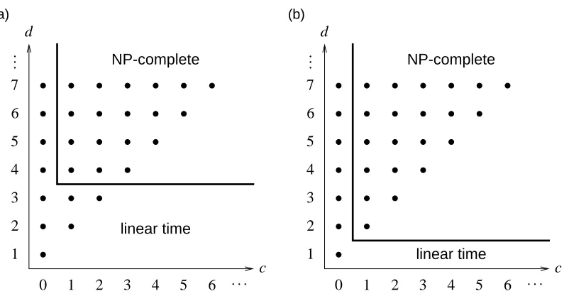
Figure 1: The dichotomies of the consistency and maximum consistency problems with coinci-dence c and sparseness d: (a) Consistency problems for the classes

B

and

B

`, where`≥2 (see Theorems 1 and 2); (b) maximum consistency problems for

B

,

B

`, where`≥1, and

L

(see Theorems 3, 4, and 5). Linear time refers to the computing time required on a RAM model with uniform measure (see Section 2.4).

Finally, we present a dichotomy theorem for maximum consistency problems regarding neurons with arbitrary weights.

Theorem 5 MAX-L-CONSISTENCY WITHCOINCIDENCEcANDSPARSENESSd is NP-complete whenever c≥1 and d≥2. On the other hand, MAX-

L

-CONSISTENCY WITH COINCIDENCE 0 and MAX-L-CONSISTENCY WITHSPARSENESSd for d≤1 is solvable in linear time.

The dichotomy theorems are illustrated in Figure 1. The dot with coordinates(c,d)represents the consistency problem or the maximum consistency problem, respectively, with coincidence c and sparseness d. Note that for c≥d the problem at coordinate(c,d)can be identified with the problem at(d−1,d)(see the discussion at the end of Section 2.3). Problems with sparseness 0 are omitted as they are trivial.

4. NP-Complete Problems

and the threshold and checking consistency or maximum consistency for the given function classes can be done in polynomial time.3

4.1 Consistency

The problem

B

-CONSISTENCYwithout sample restrictions was shown to be NP-complete by Pitt and Valiant (1988). They have defined a reduction from the problem ZERO-ONE INTEGERPRO -GRAMMING that uses samples of unbounded coincidence and, hence, unbounded sparseness. To prove the stronger result, we make a new approach and establish a reduction from a problem that is a variant of the satisfiability problem which we call ALMOSTDISJOINTPOSITIVE1-IN-3SAT.

ALMOSTDISJOINTPOSITIVE1-IN-3SAT

Instance: A set U of variables, a collection

C

of subsets of U such that each subset C∈

C

has exactly three elements and each pair of subsets C,D∈

C

,C6=D, satisfies|C∩D| ≤1.

Question: Is there a truth assignmentα: U→ {0,1}such that each subset in

C

has exactly one true variable?

The attribute “positive” refers to the fact that the variables are not negated; “almost disjoint” means that two subsets have at most one variable in common. The problem POSITIVE1-IN-3SATis known to be NP-complete (Garey and Johnson, 1979, p. 259). That the subproblem is NP-complete as well is claimed by the following statement. Its proof is given in the appendix.

Lemma 6 ALMOSTDISJOINTPOSITIVE1-IN-3SATis NP-complete.

This fact is employed in the following result. It covers the NP-completeness part of in The-orem 1. (Note that, as was argued in Section 2.3, NP-hardness of the consistency problem with coincidence c and sparseness d implies NP-hardness for any coincidence c0 ≥c and sparseness d0≥d.)

Theorem 7

B-C

ONSISTENCY WITHCOINCIDENCE1ANDSPARSENESS4 is NP-complete.

Proof The proof is by reduction from the problem ALMOSTDISJOINT POSITIVE1-IN-3SAT de-fined above. Assume that an instance of this problem is given by the set of variables U={u1, . . . ,un} and the collection of subsets

C

={c1, . . . ,cm}. The reduction maps this instance to a sample S⊆ {0,1}4n+m+2_{×{0,1}. We introduce the following notation: Given a set{i}

1, . . . ,ij} ⊆ {1, . . . ,k}, let[i1, . . . ,ij]k denote that element of{0,1}k which has a 1 in positions i1, . . . ,ij, and 0 elsewhere. Then S is constructed as follows: For each variable ui∈U , we define four examples

[i,n+i]4n+m+2 ∈ Neg(S), (1)

[2n+i,3n+i]4n+m+2 ∈ Neg(S), (2)

[i,3n+i,4n+m+2]4n+m+2 ∈ Pos(S), (3)

Position i Value of wi 1, . . . ,n α(ui) n+1, . . . ,2n 1−α(ui) 2n+1, . . . ,3n α(ui) 3n+1, . . . ,4n 1−α(ui) 4n+1, . . . ,4n+m 1

4n+m+1 1 4n+m+2 1

Table 1: Definition of the weights for a given truth assignmentα.

Each subset c`={ui,uj,uk} ∈

C

gives rise to three examples

[i,j,k,4n+`]4n+m+2 ∈ Pos(S), (5)

[n+i,n+j,n+k]4n+m+2 ∈ Pos(S), (6)

[4n+`,4n+m+2]4n+m+2 ∈ Pos(S). (7) Finally, we add the three examples

[4n+m+1]4n+m+2 ∈ Neg(S), (8)

[4n+m+2]4n+m+2 ∈ Neg(S), (9)

[4n+m+1,4n+m+2]4n+m+2 ∈ Pos(S). (10) Obviously, S can be computed from U and

C

in polynomial time. Further, as can easily be checked, we have Coin(S)≤1 and Sparse(S)≤4. (Note that every pair of different subsets in

C

has at most one common variable. Hence, the examples in (5) and (6) that arise from different subsets have coincidence at most 1.)

It remains to show that the reduction is correct, that is, that

C

has a truth assignment with exactly one true variable in each subset if and only if there exists a function in

B4n

+m+2that is consistent with S. In order to prove the “only if” part, assume thatα: U→ {0,1}is a truth assignment that satisfies the assumption. Define the weights w1, . . . ,w4nas follows: For i=1, . . . ,n, let

wi = w2n+i = α(ui), wn+i = w3n+i = 1−α(ui). The remaining weights and the threshold are determined by

w4n+1=· · ·=w4n+m+2=1 and t=2.

The representation of the truth assignment by the weights is shown in Table 1. Using the fact thatα assigns exactly one 1 to each subset in

C, it is easy to verify that the function represented by these

parameter values is consistent with S.

For establishing the “if” part, let the weights w1, . . . ,w4n+m+2∈ {0,1}and the threshold t rep-resent a function that is consistent with S. The examples in (8), (9), and (10) imply that

from which it follows that w4n+m+1=1 and w4n+m+2=1. Hence, the threshold satisfies 1<t≤2, and we may assume without loss of generality that t=2. Then the examples in (7) entail that w4n+1=· · ·=w4n+m=1. From the examples in (1) to (4) and the facts that w4n+m+2=1 and t=2, we derive the inequalities

wi+wn+i ≤ 1, w2n+i+w3n+i ≤ 1, wi+w3n+i ≥ 1, wn+i+w2n+i ≥ 1, for i=1, . . . ,n. These imply the equalities

wi+wn+i = 1, (11)

for i=1, . . . ,n. We define the truth assignmentα: U→ {0,1}by

α(ui) = wi,

for i=1, . . . ,n. The examples in (5), (6) and the fact that t=2 yield the inequalities

wi+wj+wk+w4n+` ≥ 2,

wn+i+wn+j+wn+k ≥ 2,

for each subset c`={ui,uj,uk} ∈

C

. From these, the fact that w4n+1=· · ·=w4n+m=1, and the equations (11) we get that c`satisfies

α(ui) +α(uj) +α(uk) = 1.

Thus, each subset in

C

has exactly one 1 assigned byα. This completes the correctness proof for the reduction.

The foregoing proof shows that the same reduction can be used whenever the threshold is al-lowed to take on the value 2. Thus, it follows that the problems in Theorem 7 are NP-complete also for neurons with threshold at most`, where`≥2. This observation establishes the NP-completeness statement of Theorem 2.

Corollary 8 For every`≥2,

B

`-CONSISTENCY WITH COINCIDENCE1 AND SPARSENESS4 is NP-complete.

4.2 Maximum Consistency

Now, we address the NP-completeness of the maximum consistency problems. The following result covers the intractability part of Theorem 3.

Proof H¨offgen et al. (1995) have shown that the maximum consistency problem for the class

L

and for samples without restrictions is NP-complete. They constructed a reduction from VERTEX COVER(Garey and Johnson, 1979, p. 190). This is the problem to decide, given a graph G= (V,E)

and a number k, whether there exists a set V0⊆V with|V0| ≤k such that for each edge{u,v} ∈E at least one of u and v belongs to V0. We use this problem for the reduction, too, but we take account of the fact that the weights are from the set{0,1}.

Let (V,E) and k be an instance of VERTEX COVER, where V ={v1, . . . ,vn}. We define the sample S⊆ {0,1}2n_{× {0,1} using the notation introduced in the proof of Theorem 7. For each} vi∈V , there is a “vertex example”

[i,n+i]2n ∈ Neg(S). Each e={vi,vj} ∈E results in two “edge examples”

[i,j]2n ∈ Pos(S),

[n+i,n+j]2n ∈ Pos(S).

The cardinality of the subsample in the instance of the maximum consistency problem is set to the value |S| −k. It is obvious that Coin(S)≤1 and Sparse(S)≤2 holds, and that the reduction is computable in polynomial time.

We claim that (V,E) has a vertex cover of cardinality at most k if and only if there exists a function in

B2n

that is consistent with at least|S| −k examples. Let V0⊆V be a vertex cover with at most k elements. Define the weights w1, . . . ,w2nby

wi = wn+i =

1 if vi∈V0, 0 otherwise,

for i=1, . . . ,n, and let the threshold be t =1. Then, the vertex example [i,n+i]2n is classified correctly if and only if vi∈V\V0. Further, since V0is a vertex cover, all edge examples are classified correctly. Thus, the function computed by this neuron is consistent with at least|S| −k elements.

On the other hand, let the weights w1, . . . ,w2n and the threshold t represent a function that is consistent with a subsample of S of cardinality at least|S| −k. Define a set V0of vertices as follows: For each vertex example that is classified wrongly include the corresponding vertex in V0; for each edge example that is classified wrongly arbitrarily choose one of the vertices the edge is incident with and include it in V0. Consequently, V0 contains at most k elements. In order to show that V0 is a vertex cover, assume that{vi,vj} ∈E is not covered, that is, we have{vi,vj} ∩V0= /0. Then, by the construction of V0, the function is consistent with the two vertex examples that arose from vi and vj, and it is consistent with the two edge examples due to{vi,vj}. Thus, we get

wi+wn+i+wj+wn+j < 2t,

wi+wj+wn+i+wn+j ≥ 2t,

a contradiction. This implies that V0is a vertex cover.

Corollary 10 For every`≥1, MAX-B`-CONSISTENCY WITH COINCIDENCE1 ANDSPARSE -NESS2 is NP-complete.

Furthermore, we observe that the proof of Theorem 9 does not make use of the assumption that the weights must be from the set{0,1}. Consequently, the reduction works also for uncon-strained weights, that is, for the function class

L. This establishes the NP-completeness statement

of Theorem 5.

Corollary 11 MAX-

L

-CONSISTENCY WITHCOINCIDENCE1ANDSPARSENESS2 is NP-complete.

5. Problems Solvable in Linear Time

In the following, we show that all consistency problems and maximum consistency problems not yet considered in the foregoing section have algorithms that run in linear time on a RAM as made precise in Section 2.4. Thus, if P6=NP holds, the values of coincidence and sparseness established in the NP-completeness results are optimal. Moreover, as any algorithm that solves a consistency or maximum consistency problem must pass through the entire sample, the linear-time bound cannot be improved either. Thus, we not only obtain a complete characterization of the complexity of consistency problems for the function classes

B

,

B

`, and

L

with sample restrictions, but also reveal the striking fact that, with respect to the RAM computer model, these classes consist solely of problems of the lowest and highest complexity in NP. All algorithms presented here are constructive, that is, they solve the decision problem by computing a solution if one exists.

5.1 Consistency

It is convenient to begin with the consistency problem for neurons with a bounded threshold. The case that remains to be considered is the function class

B

1. The result for this class implies the second part of Theorem 2. It is valid for samples with arbitrary coincidence and sparseness.

Theorem 12

B

1-CONSISTENCYis solvable in linear time.

Proof If there are weights w1, . . . ,wn∈ {0,1} and a threshold t∈ {0,1} consistent with a given sample S then we may set t=0 if Neg(S) = /0. On the other hand, if S contains negative examples, we must have t=1. Then we ensure that w·x=0 for all x∈Neg(S). These are the steps performed by Algorithm 1, which is basically the standard consistency algorithm for disjunctions. The most time consuming part is the for-loop in lines 8–12. It is obvious that this statement can be imple-mented such that it requires no more than linear time on a RAM.

It is easy to see that if some function in

B

is consistent with a sample S that has coincidence 0, the threshold can be chosen to satisfy t≤1. Therefore, Algorithm 1 solves also the problem

B

-CONSISTENCY WITHCOINCIDENCE0.

Corollary 13

B

-CONSISTENCY WITHCOINCIDENCE0 is solvable in linear time.

Algorithm 1

B

1-CONSISTENCY Input: sample S⊆ {0,1}n_{× {0,1}}

Output: w1, . . . ,wn,t 1: for i=1, . . . ,n do

2: wi:=1 3: end for;

4: if Neg(S) =/0then 5: t :=0;

6: else 7: t :=1;

8: for all x∈Neg(S)do

9: if there is some i∈ {1, . . . ,n}with xi=1 then 10: wi:=0

11: end if 12: end for 13: end if.

Theorem 14

B

-CONSISTENCY WITHSPARSENESS3 is solvable in linear time.

Proof We show that Algorithm 2 computes a solution for samples with sparseness 3 provided

that one exists. Without loss of generality we may assume that the threshold satisfies t≤3. The algorithm has three parts that correspond to the possible values for the threshold: t≤1, t=3, and t=2. In lines 1–2 Algorithm 1 is used to check whether there is a function in the class

B

1consistent with S.

If this fails, the algorithm assumes in lines 3–12 that t=3. Here, the assignment of values to the weights is based on the fact that every positive example must reach the threshold. Hence, its non-zero components, of which there must be exactly three, specify which weights receive the value 1.

In the last part, starting from line 13, we can only have that t =2. We show that this case of the consistency problem can be solved via a 2-SATISFIABILITYproblem. The algorithm maps the sample S to a set

C

of clauses over the variables w1, . . . ,wn. Each clause has at most two literals of the form wi or¬wi. For each element x∈Dom(S)the set

C

is augmented with clauses that depend on the properties of x. Lines 17–23 deal with the case that x has a 1 in exactly three positions. If x is a positive example then no two weights at these positions may both be equal to 0. This is expressed by the three clauses in line 20. If x is a negative example then no two of these weights may both be equal to 1. This is taken into account by adding the three clauses in line 22. Lines 24–30 treat the examples with exactly two 1s. If x is positive then both weights must be equal to 1 (line 27); if x is negative then at least one weight must be 0 (line 29). Finally, if x has at most one non-zero position and x is positive then the consistency problem has no solution. This is taken care of in line 34 by adding two contradictory clauses. On the other hand, if x is negative then it will be classified as such and nothing needs to be done. In the last step an algorithm for 2-SATISFIABILITYis called with the constructed set of clauses as input.

Algorithms that compute satisfying assignments for 2-SATISFIABILITYproblems in linear time on a RAM with uniform measure have been designed by Even et al. (1976) and Aspvall et al. (1979). It is obvious that the size of the constructed instance for 2-SATISFIABILITYis at most linear in the size of the sample. Thus, line 38 can be executed in linear time. We conclude that the running time of Algorithm 2 on a random access machine is linear.

With the previous result the proof of Theorem 1 is completed. Obviously, Algorithm 2 solves also the consistency problems with sparseness 3 for the classes

B

`where`≥2. (If`=2, the middle part of the algorithm, which assumes t=3, is needless.) Furthermore, if some function in

B

` is consistent with a sample having coincidence 0 then there is also some function in

B

1 consistent with that sample. Consequently, Algorithm 1 solves also the problems

B

`-CONSISTENCY WITH COINCIDENCE0 for every`≥2. Hence, Theorems and 14 and 12 yield the following statement. It finalizes the proof of Theorem 2.

Corollary 15 For every`≥2,

B

`-CONSISTENCY WITHCOINCIDENCE0 and

B

`-CONSISTENCY WITHSPARSENESS3 is solvable in linear time.

5.2 Maximum Consistency

At last, we give attention to the maximum consistency problems that are claimed as linear-time solvable in Theorems 3, 4, and 5. The main issues that have to be dealt with are contradictory pairs and examples that are 0 in all positions. With the first result we finish the proof of Theorem 3.

Theorem 16 The problems MAX-B-CONSISTENCY WITHCOINCIDENCE0 and MAX-B-CONSISTENCY WITHSPARSENESS1 are solvable in linear time.

Proof If Neg(S) = /0 then by letting w1 =· · ·=wn=0 and t =0 we obtain the function that always outputs 1, which is consistent with all examples. Assume now that Neg(S)6= /0. Algorithm 3 generates a function that has the following properties: For each example x∈Dom(S) that is part of a contradictory pair, that is, where(x,0)∈S and (x,1)∈S, the function is consistent with the positive example. Further, it is consistent with all examples that are not part of a contradictory pair, except possibly for the example(0, . . . ,0)∈Pos(S)\Neg(S), which is classified as negative. It is obvious that this is the maximum number of examples that can be classified correctly, unless

(0, . . . ,0)∈Pos(S)\Neg(S)is the only example that is not part of a contradictory pair. In this case we can increase the number of correctly classified examples by using the function that constantly outputs 1, which is then consistent with the positive example in each contradictory pair and with

(0, . . . ,0)∈Pos(S).

It is obvious that Algorithm 3 and the additional steps described above require no more than linear time on a RAM. In particular, whether (0, . . . ,0) is the only example that is not part of a contradictory pair can be checked in linear time using radix sort.

Algorithm 2

B

-CONSISTENCY Input: sample S⊆ {0,1}n_{× {0,1}}

Output: w1, . . . ,wn,t

1: get w1, . . . ,wn,t from

B

1-CONSISTENCY(S);

2: if(w1, . . . ,wn,t)is consistent with S then stop end if; 3: t :=3;

4: for i=1, . . . ,n do

5: wi:=0 6: end for;

7: for all x∈Pos(S)do

8: if there is some x∈Pos(S)with xi=1 then 9: wi:=1

10: end if 11: end for;

12: if(w1, . . . ,wn,t)is consistent with S then stop end if; 13: t :=2;

14:

C

:=/0;

15: for all x∈Dom(S)do{construct a set

C

of clauses over w1, . . . ,wn} 16: let I={i|xi=1};

17: if|I|=3 then 18: let{j,k, `}=I;

19: if x∈Pos(S)then

20:

C

:=

C

∪

{wj,wk},{wj,w`},{wk,w`} 21: else{we have x∈Neg(S)}

22:

C

:=

C

∪

{¬wj,¬wk},{¬wj,¬w`},{¬wk,¬w`} 23: end if

24: else if|I|=2 then 25: let{j,k}=I;

26: if x∈Pos(S)then

27:

C

:=

C

∪

{wj},{wk} 28: else{we have x∈Neg(S)}

29:

C

:=

C

∪

{¬wj,¬wk} 30: end if

31: else{we have|I| ≤1}

32: if |I|=1 then let{j}=I else j :=1 end if; 33: if x∈Pos(S)then

34:

C

:=

C

∪

{wj},{¬wj} 35: end if

36: end if 37: end for;

38: get w1, . . . ,wnfrom 2-SATISFIABILITY({w1, . . . ,wn},

C

).

Algorithm 3 MAX-

B

-CONSISTENCY Input: sample S⊆ {0,1}n_{× {0,1}}

Output: w1, . . . ,wn,t t :=1;

for i=1, . . . ,n do wi:=0

end for;

for all x∈Pos(S)do

if there is some i∈ {1, . . . ,n}with xi=1 then wi:=1

end if end for.

Corollary 17 For every `≥1, MAX-B`-CONSISTENCY WITH COINCIDENCE 0 and MAX-B` -CONSISTENCY WITHSPARSENESS1 is solvable in linear time.

The following result completes the proof of Theorem 4.

Lemma 18 MAX-B0-CONSISTENCYis solvable in linear time.

Proof If the threshold is equal to 0 then everything is classified as positive regardless of which

values the weights may have. Thus, outputting any weights and t =0 provides a solution if one exists. For solving the decision problem, observe that consistency with at least k examples in S is equivalent to the condition|Pos(S)| ≥k. This can clearly be checked in linear time on a RAM.

Finally, we prove the remaining part of Theorem 5 that claims linear time bounds.

Theorem 19 The problems MAX-L-CONSISTENCY WITHCOINCIDENCE0 and MAX-L-CONSISTENCY WITHSPARSENESS1 are solvable in linear time.

Proof Consider Algorithm 4 for inputs satisfying Coin(S) =0. If Neg(S) = /0then the resulting function is consistent with all examples. In the case that Neg(S)6=/0holds we argue as in the proof of Theorem 16: For every contradictory pair, the function is consistent with the positive example. Further, it is consistent with every example that is not part of a contradictory pair. (In contrast to the proof of Theorem 16, this holds also in all cases where(0, . . . ,0)∈Dom(S) due to the use of negative weights by Algorithm 4.) Clearly, this is the maximum number of examples a function can be consistent with.

Since any subsample S0 of S that contains no contradictory pairs must satisfy Coin(S0) =0 if Sparse(S) =1, Algorithm 4 solves also the maximum consistency problem for samples with sparseness 1.

Algorithm 4 MAX-L-CONSISTENCY Input: sample S⊆ {0,1}n_{× {0,1}}

Output: w1, . . . ,wn,t

if(0, . . . ,0)∈Pos(S)then

t :=0

else

t :=1

end if;

for i=1, . . . ,n do wi:=−1

end for;

for all x∈Pos(S)do

if there is some i∈ {1, . . . ,n}with xi=1 then wi:=1

end if end for.

6. Conclusions

With this work we aimed at providing necessary and sufficient conditions for the existence of effi-cient learning algorithms. The approach that we have taken is to consider criteria for the complexity of samples and to use them for the definition of subproblems. As results we obtained dichotomy theorems that completely characterize the dividing lines between the polynomial-time solvable and the NP-complete problems.

An NP-completeness assertion is a worst-case result stating that, if P 6=NP then there is no algorithm that solves the problem in polynomial time for all instances. One way to cope with intractability is therefore trying to avoid instances that make the problem hard. This gives rise to subproblems that may be more appropriate to practical situations where one often needs not deal with all possible instances but only a subset thereof. The results here show that such deliberations can indeed lead to the discovery of new efficient learning algorithms. While it is not clear whether the restrictions they suppose are always met in applications, these algorithms could be helpful in the development of better heuristics for more general learning problems.

Acknowledgments

I thank the anonymous reviewers for their helpful comments and suggestions. This work was sup-ported in part by the IST Programme of the European Community, under the PASCAL Network of Excellence, IST-2002-506778.

Appendix A. An NP-Complete Satisfiability Problem

Lemma 6 in Section 4.1 claims that the problem ALMOSTDISJOINTPOSITIVE1-IN-3SAT intro-duced in that section is NP-complete. Here we give a proof of this statement.

Lemma 6 ALMOSTDISJOINTPOSITIVE1-IN-3SATis NP-complete.

Proof It is clear that the problem is in NP. To prove its NP-hardness, we construct a reduction from

POSITIVE 1-IN-3SAT. In this variant of the problem the requirement is missing that two subsets have at most one variable in common. The idea of the reduction is to establish the property of almost disjointness by introducing new variables as substitutes for old ones. The correctness of the reduction is ensured by augmenting the collection with additional subsets.

Let

C

be the collection of subsets from the instance of POSITIVE 1-IN-3SAT. Further, let C,D∈

C

be two subsets with two common variables, say C={u1,u2,u3}and D={u1,u2,u4}. We introduce a set of new variables V ={v1, . . . ,v5}, replace in D the variable u1by v1and join

C

with the collection

D

defined as

D

=

{v1,v2,v3}, {v1,v4,v5},{u1,v2,v4}, {u1,v3,v5} .

Obviously, no pair of subsets in

D

has more than one common variable. Further, no subset in

D

has more than one variable in common with any subset in

C

. Hence, going from

C

to

C

∪

D, the

number of pairs that violate the condition of almost disjointness decreases by one.

We say that a truth assignment is a 1-IN-3SAT assignment for a collection of subsets if each subset has exactly one true variable. Let U be the set of variables in

C

. We claim that the following two conditions hold:

(A.1) Every 1-IN-3SAT assignmentα: U → {0,1}for

C

can be extended to a 1-IN -3SATassignmentα: U∪V → {0,1}for

C

∪

D

satisfyingα(u1) =α(v1). (A.2) Every 1-IN-3SAT assignment α: U∪V → {0,1} for

C

∪

D

satisfies α(u1) =

α(v1).

That condition (A.1) is valid can be seen as follows: Givenα defined on U , we letα(v1) =α(u1) and extend it to the remaining variables of V in the following way: In the case α(u1) =0 we defineα(v2) =α(v5) =0 andα(v3) =α(v4) =1; in the case α(u1) =1 we letα(v2) =α(v3) = α(v4) =α(v5) =0. For the proof of condition (A.2) we observe that ifα(v1) =1, we must have α(v2) =α(v3) =α(v4) =α(v5) =0 due to the first two subsets in

D

, and hence, because of the last two subsets,α(u1) =1; on the other hand, ifα(u1) =1, analogous reasoning yields thatα(v1) =1 must hold. Thus, u1and v1cannot have different truth values assigned byα.

the reduction follows inductively. It is obvious that the reduction is computable in polynomial time. Thus, ALMOSTDISJOINTPOSITIVE1-IN-3SATis NP-hard.

References

Amaldi, E. (1991). On the complexity of training Perceptrons. In Kohonen, T., M ¨akisara, K., Sim-ula, O., and Kangas, J., editors, Artificial Neural Networks, pages 55–60. Elsevier, Amsterdam.

Anthony, M. and Bartlett, P. L. (1999). Neural Network Learning: Theoretical Foundations. Cam-bridge University Press, CamCam-bridge.

Aspvall, B., Plass, M. F., and Tarjan, R. E. (1979). A linear-time algorithm for testing the truth of certain quantified Boolean formulas. Information Processing Letters, 8:121–123.

Blum, A. L. and Rivest, R. L. (1992). Training a 3-node neural network is NP-complete. Neural Networks, 5:117–127.

Blumer, A., Ehrenfeucht, A., Haussler, D., and Warmuth, M. K. (1989). Learnability and the Vapnik-Chervonenkis dimension. Journal of the Association for Computing Machinery, 36:929– 965.

Cook, S. A. and Reckhow, R. A. (1973). Time bounded random access machines. Journal of Computer and System Sciences, 7:354–375.

Dalmau, V. (1999). A dichotomy theorem for learning quantified Boolean formulas. Machine Learning, 35:207–224.

Dalmau, V. and Jeavons, P. (2003). Learnability of quantified formulas. Theoretical Computer Science, 306:485–511.

Even, S., Itai, A., and Shamir, A. (1976). On the complexity of timetable and multicommodity flow problems. SIAM Journal on Computing, 5:691–703.

Fang, S. C. and Venkatesh, S. S. (1996). Learning binary Perceptrons perfectly efficiently. Journal of Computer and System Sciences, 52:374–389.

Garey, M. R. and Johnson, D. S. (1979). Computers and Intractability: A Guide to the Theory of NP-Completeness. W. H. Freeman, San Francisco.

Golea, M. and Marchand, M. (1993). On learning Perceptrons with binary weights. Neural Com-putation, 5:767–782.

Hampson, S. E. and Volper, D. J. (1986). Linear function neurons: Structure and training. Biological Cybernetics, 53:203–217.

H¨offgen, K.-U., Simon, H.-U., and Van Horn, K. S. (1995). Robust trainability of single neurons. Journal of Computer and System Sciences, 50:114–125.

Judd, J. S. (1990). Neural Network Design and the Complexity of Learning. The MIT Press, Cambridge, MA.

Kearns, M. J., Schapire, R. E., and Sellie, L. M. (1994). Toward efficient agnostic learning. Machine Learning, 17:117–141.

Kim, J. H. and Roche, J. R. (1998). Covering cubes by random half cubes, with applications to binary neural networks. Journal of Computer and System Sciences, 56:223–252.

Kirousis, L. M. and Kolaitis, P. G. (2003). The complexity of minimal satisfiability problems. Information and Computation, 187:20–39.

Littlestone, N. (1988). Learning quickly when irrelevant attributes abound: A new linear-threshold algorithm. Machine Learning, 2:285–318.

Maass, W. and Tur´an, G. (1994). How fast can a threshold gate learn? In Hanson, S. J., Drastal, G., and Rivest, R., editors, Computational Learning Theory and Natural Learning Systems: Con-straints and Prospects, pages 381–414. The MIT Press, Cambridge, MA.

McCulloch, W. S. and Pitts, W. (1943). A logical calculus of the ideas immanent in nervous activity. Bulletin of Mathematical Biophysics, 5:115–133.

Natarajan, B. K. (1991). Machine Learning: A Theoretical Approach. Morgan Kaufmann, San Mateo, CA.

Palm, G. (1980). On associative memory. Biological Cybernetics, 36:19–31.

Pitt, L. and Valiant, L. G. (1988). Computational limitations on learning from examples. Journal of the Association for Computing Machinery, 35:965–984.

Schaefer, T. J. (1978). The complexity of satisfiability problems. In Proceedings of the 10th Annual ACM Symposium on Theory of Computing, pages 216–226.

Schmitt, M. (1994a). On the complexity of consistency problems for neurons with binary weights. Ulmer Informatik-Berichte 94-01, Universit¨at Ulm.

Schmitt, M. (1994b). On the size of weights for McCulloch-Pitts neurons. In Caianiello, E. R., editor, Proceedings of the Sixth Italian Workshop on Neural Nets WIRN VIETRI-93, pages 241– 246, World Scientific, Singapore.

Schmitt, M. (1995). On methods to keep learning away from intractability. In Fogelman-Souli ´e, F. and Gallinari, P., editors, Proceedings of the International Conference on Artificial Neural Networks ICANN ’95, volume 1, pages 211–216, EC2 & Cie., Paris.

Sommer, F. T. and Palm, G. (1999). Improved bidirectional retrieval of sparse patterns stored by Hebbian learning. Neural Networks, 12:281–297.

van Emde Boas, P. (1990). Machine models and simulations. In van Leeuwen, J., editor, Handbook of Theoretical Computer Science, volume A: Algorithms and Complexity, chapter 1, pages 1–66. Elsevier, Amsterdam.

ˇS´ıma, J. (2002). Training a single sigmoidal neuron is hard. Neural Computation, 14:2709–2728.