Kernel Method for Persistence Diagrams via Kernel
Embedding and Weight Factor
Genki Kusano [email protected]
Graduate School of Science Tohoku University
Sendai, Miyagi 980-8578, Japan
Kenji Fukumizu [email protected]
The Institute of Statistical Mathematics Tachikawa, Tokyo 190-8562, Japan
Yasuaki Hiraoka [email protected]
Advanced Institute for Materials Research Tohoku University
Sendai, Miyagi 980-0811, Japan
Editor:Arthur Gretton
Abstract
Topological data analysis (TDA) is an emerging mathematical concept for characteriz-ing shapes in complicated data. In TDA, persistence diagrams are widely recognized as a useful descriptor of data, distinguishing robust and noisy topological properties. This pa-per introduces a kernel method for pa-persistence diagrams to develop a statistical framework in TDA. The proposed kernel is stable under perturbation of data, enables one to explicitly control the effect of persistence by a weight function, and allows an efficient and accurate approximate computation. The method is applied into practical data on granular systems, oxide glasses and proteins, showing advantages of our method compared to other relevant methods for persistence diagrams.
Keywords: topological data analysis, persistence diagrams, kernel method, kernel em-bedding, persistence weighted Gaussian kernel
1. Introduction
Recent years have witnessed an increasing interest in utilizing methods of algebraic topology for statistical data analysis. In terms of algebraic topology, conventional clustering meth-ods are regarded as charactering 0-dimensional topological features which mean connected components of data. Furthermore, higher dimensional topological features also represent informative shape of data, such as rings (1-dimension) and cavities (2-dimension). The re-search analyzing these topological features in data is calledtopological data analysis(TDA) (Carlsson, 2009), which has been successfully applied to various areas including information science (Carlsson et al., 2008; de Silva and Ghrist, 2007), biology (Kasson et al., 2007; Xia and Wei, 2014), brain science (Lee et al., 2011; Petri et al., 2014; Singh et al., 2008), bio-chemistry (Gameiro et al., 2015), material science (Hiraoka et al., 2016; Nakamura et al., 2015; Saadatfar et al., 2017), and so on. In many of these applications, data have
com-c
plicated geometric structures, and thus it is important to extract informative topological features from the data.
A persistent homology(Edelsbrunner et al., 2002), which is a key mathematical tool in TDA, extracts robust topological information from data, and it has a compact expression called apersistence diagram. While it is applied to various problems such as the ones listed above, statistical or machine learning methods for analysis on persistence diagrams are still limited. In TDA, analysts often elaborate only single persistence diagram and, in particular, methods for handling many persistence diagrams, which can contain randomness from the data, are at the beginning stage (see the end of this section for related works). Hence, developing a framework of statistical data analysis on persistence diagrams is a significant issue for further success of TDA and, to this goal, this paper discusses kernel methods for persistence diagrams.
1.1 Topological Descriptor
In order to provide some intuitions for the persistent homology, let us consider a typical way of constructing persistent homology from data points in a Euclidean space, assuming that the point set lies on a submanifold. The aim is to make inference on the topology of the underlying manifold from finite data points. We consider the r-balls (balls with radiusr) to recover the topology of the manifold, as popularly employed in constructing an r-neighbor graph in many manifold learning algorithms. While it is expected that, with an appropriate choice ofr, ther-ball model can represent the underlying topological structures of the manifold, it is also known that the result is sensitive to the choice ofr. Ifris too small (resp. large), the union ofr-balls consists simply of the disjointr-balls (resp. a contractible space). Then, by considering not one specific r but all r, the persistent homology gives robust topological features of the point set.
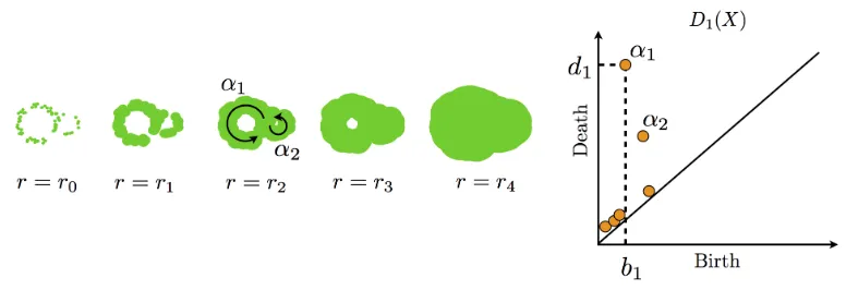
As a useful representation of persistent homology, a persistence diagram is often used in topological data analysis. The persistence diagram is given in the form of a multiset D = {(bi, di) ∈ R2 | i ∈ I, bi < di} (Figure 1). Every point (bi, di) ∈ D, called a
generator of the persistent homology, represents a topological property (e.g., connected components, rings, cavities, etc.) which appears at r = bi and disappears at r = di in
the ball model. Then, the persistencedi−bi of the generator shows the robustness of the
topological property under the radius parameter. A generator with large persistence can be regarded as a reliable structure, while that with small persistence (points close to the diagonal) is likely to be a structure caused by noise. In this way, persistence diagrams encode topological and geometric information of data points.
1.2 Contributions
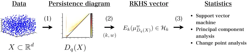
Since a persistence diagram is a point set of variable size, it is not straightforward to apply standard methods of statistical data analysis, which typically assume vectorial data. To vectorize persistence diagrams, we employ the framework of kernel embedding of (prob-ability and more general) measures into reproducing kernel Hilbert spaces (RKHS). This framework has recently been developed and leading various new methods for nonparamet-ric inference (Muandet et al., 2017; Smola et al., 2007; Song et al., 2013; Lopez-Paz et al., 2015; Szab´o et al., 2016). It is known (Sriperumbudur et al., 2011) that, with an appropri-ate choice of kernels, a signed Radon measure can be uniquely represented by the Bochner integral of the feature vectors with respect to the measure. Since a persistence diagram can be regarded as a sum of Dirac delta measures, it can be embedded into an RKHS by the Bochner integral. Once such a vector representation is obtained, we can introduce any kernel methods for persistence diagrams systematically (see Figure 2).
Overview of this talk
0 5 10 15 20 25 0 5 10 15 20 250 5 10 15 20 25 30
[˚A2]
[
˚A
2]
−0.50 0 0.5 1 1.5 2 2.5 3 0.5 1 1.5 2 2.5 3 Multiplicity 0.2 0.4 0.6 0.8 1 1.2 1.4 1.6 1.8 2
D
q(
X
)
X
⇢
R
dEk(µwDq(X))2 Hk (k, w)
Persistence diagram
Data RKHS vector
• Support vector machine
• Principal component analysis
• Change point analysis
Statistics
(1) (2) (3)
Figure 2: (1) A data set X is transformed into a persistence diagram Dq(X) (Section 2.1).
(2) The persistence diagramDq(X) is mapped to an RKHS vectorEk(µwDq(X)),
where k is a positive definite kernel and w is a weight function controlling the effect of persistence (Section 3.1). (3) Statistical methods are applied to those vector representations of persistence diagrams (Section 4).
advantages of this kernel are as follows: (i) We can explicitly control the effect of persistence by a weight function, and hence discount the noisy generators appropriately in statistical analysis. (ii) As a theoretical contribution, the distance defined by the RKHS norm for the PWGK satisfies the stability property, which ensures the continuity from data to the vector representation of the persistence diagram. (iii) The PWGK allows efficient computation by using the random Fourier features (Rahimi and Recht, 2007), and thus it is applicable to persistence diagrams with a large number of generators.
We demonstrate the performance of the proposed kernel method with synthesized and real-world data, including granular systems (taken by X-ray Computed Tomography on granular experiments), oxide glasses (taken by molecular dynamics simulations) and protein data set (taken by NMR and X-ray crystallography experiments). We remark that these real-world problems have physical and biochemical significance in their own right, as detailed in Section 4.
1.3 Related Works
There are already some relevant works on statistical approaches to persistence diagrams. Some studies discuss how to transform a persistence diagram to a vector (Bubenik, 2015; Reininghaus et al., 2015; Adams et al., 2017; Cang et al., 2015; Robins and Turner, 2016; Donatini et al., 1998). In these methods, a transformed vector is typically expressed in a Euclidean space Rk or a function space Lp, and simple and ad-hoc summary statistics
like means and variances are used for data analysis such as principal component analysis (PCA) and support vector machines (SVMs). In this paper, we will compare the perfor-mance among the PWGK, the persistence scale-space kernel (Reininghaus et al., 2015), the persistence landscape (Bubenik, 2015), the persistence image (Adams et al., 2017), and the molecular topological fingerprint (Cang et al., 2015) in several machine learning tasks. Furthermore, we show that our vectorization is a generalization of the persistence scale-space kernel and the persistence image although the constructions are different. We also remark that there are some works discussing statistical properties of persistence diagrams for random data points: Chazal et al. (2015) show convergence rates of persistence diagram estimation, and Fasy et al. (2014) discuss confidence sets in a persistence diagram. These works consider a different but important direction to the statistical methods for persistence diagrams.
The remaining of this paper is organized as follows: In Section 2, we review some basics on persistence diagrams and kernel embedding methods. In Section 3, the PWGK is proposed, and some theoretical and computational issues are discussed. Section 4 shows experimental results and compares the proposed kernel method with other methods.
2. Backgrounds
We review the concepts of persistence diagrams and kernel methods. For readers who are not familiar with algebraic topology, we give a brief summary in Appendix A. See also Hatcher (2002) as an accessible introduction to algebraic topology.
2.1 Persistence Diagram
In order to define a persistence diagram, we transform a data setXinto a filtrationFilt(X) and compute its persistent homologyHq(Filt(X)). In this section, we will first introduce this
mathematical framework of persistence diagrams. Then, by using a ball model filtration, we will intuitively explain geometrical meanings of persistence diagrams. The ball model filtrations can be generalized toward two constructions using ˇCech complexes and sub-level sets. The former construction is useful for computations of persistence diagrams and the latter is useful to discuss theoretical properties.
2.1.1 Mathematical Framework of Persistence Diagrams
Let K be a coefficient field of homology.1 LetFilt = {F
a|a∈R} be a (right continuous)
filtrationof simplicial complexes, i.e.,Fais a subcomplex ofFb fora≤band Fa=
T
a<bFb.
Alternatively, Filt may be a filtration of topological spaces: in this case Fa is a subspace
of Fb with the same condition as above. For a ≤ b, the K-linear map induced from the
inclusionFa,→Fb is denoted byρba:Hq(Fa)→Hq(Fb), whereHq(Fa) is theq-th homology
ofFa. Theq-thpersistent homology Hq(Filt) = (Hq(Fa), ρba) ofFilt is defined by the family
of homology {Hq(Fa)|a∈R} and the induced linear maps{ρba|a≤b}.
A homological critical value of Hq(Filt) is the number a∈ R such that the linear map
ρaa+−εε : Hq(Fa−ε) → Hq(Fa+ε) is not isomorphic for any sufficiently small ε > 0. The
persistent homology Hq(Filt) is called tame if dimKHq(Fa) < ∞ for any a ∈ R and the
number of homological critical values is finite. A tame persistent homologyHq(Filt) has a
nice decomposition property:
Theorem 1 (Zomorodian and Carlsson (2005)) A tame persistent homology can be uniquely expressed by
Hq(Filt)∼=
M
i∈I
I[bi, di], (1)
where I[bi, di] = (Ua, ιba) consists of a family of K-vector spaces
Ua=
K, bi≤a < di
0, otherwise , and ιb
a= idK for bi≤a≤b < di.2
1. In this setting, all homology areK-vector spaces. You may simply consider the case K =R, but the theory is built with an arbitrary field.
Each summand I[bi, di] means a topological feature in Filt that appears at a=bi and
disappears ata=di. The birth-death pairx= (bi, di) is called ageneratorof the persistent
homology, and pers(x) :=di−bi apersistence ofx. We note that, when dimKHq(Fa)6= 0
for anya <0 (resp. for anya >0), the decomposition (1) should be understood in the sense that some bi takes the value −∞ (resp. di = ∞), where −∞,∞ are the elements in the
extended real R=R∪ {−∞,∞}. Through the decomposition in Theorem 1, a persistent homology Hq(Filt), which is an algebraic object and is not suitable to be analyzed by
statistical methods, is transformed into a multi-set of 2-dimensional vectors Dq(Filt) =
n
(bi, di)∈R
2 i∈I
o
and we call it thepersistence diagram ofFilt.3
In this paper, we assume that all persistence diagrams have finite cardinality because a tame persistent homology defines a finite persistence diagram. Moreover, we also assume that all birth-death pairs are bounded, that is, all elements in a persistence diagram take neither ∞ nor −∞.4 In the following, we also use abstract persistence diagrams (denoted by DorE) given by finite multi-sets above the diagonal R2
ad :={(b, d)∈R2 |b < d}.
2.1.2 Ball Model Filtrations
The example used in Figure 1 can be expressed as follows. LetX={x1, . . . ,xn}be a finite
subset in a metric space (M, dM) and Xa := Sni=1B(xi;a) be a union of balls B(xi;a) =
{x∈ M |dM(xi,x) ≤a} with radius a≥0. For convenience, letXa := ∅ (a < 0). Since X={Xa|a∈R}is a right-continuous filtration of topological spaces andX is a finite set,
Hq(X) is tame and the persistence diagramDq(X) is well-defined. For notational simplicity,
the persistence diagram of this ball model filtration is denoted by Dq(X).
We remark that, in this model, there is only one generator in D0(X) that does not disappear in the filtration; its lifetime is ∞. From now on, we deal with D0(X) by re-moving this infinite lifetime generator.5 Let diam(X) be the diameter of X defined by maxxi,xj∈XdM(xi,xj). Then, all generators appear after a = 0 and disappear before
a= diam(X) because Xdiam(X) becomes a contractible space. Thus, for any dimension q, all birth-death pairs of Dq(X) have finite values.
2.1.3 Geometric Complexes
We review some standard methods of constructing a filtration from finite sets in a metric space. See also Chazal et al. (2014) for more details.
Let (M, dM) be a metric space andX ={x1, . . . ,xn}be a finite subset inM. For a fixed a≥0, we form aq-simplex [xi0· · ·xiq] as a subset{xi0, . . . ,xiq}ofXwhenever there exists
¯
x ∈ M such that dM(xij,x¯) ≤ a for all j = 0, . . . , q, or equivalently, ∩ q
j=0B(xij;a) 6= ∅.
The set of these simplices forms a simplicial complex, called the ˇCech complex of X with parameter a, denoted by ˇCech(X;a). For a < 0, we define ˇCech(X;a) as an empty set.
3. Amulti-setis a set with multiplicity of each point. We regard a persistence diagram as a multi-set, since several generators can have the same birth-death pairs.
Since there is a natural inclusion ˇCech(X;a),→Cech(ˇ X;b) whenever a ≤ b, ˇCech(X) =
ˇ
Cech(X;a) a∈R is a filtration. When M is a subspace of Rd, from the nerve lemma
(Hatcher, 2002), it is known that the topology of ˇCech(X;a) is the same asXa(Figure 3)6,
and henceDq( ˇCech(X)) =Dq(X).
As a similar concept to the ˇCech complex, the Rips complex (or Vietoris-Rips complex) is also often used in TDA. While the Rips complex gives different topology from the ˇCech complex, it can be computed much more efficiently; the Rips complex needs only pairwise distances, while the ˇCech complex needs all the (q+ 1)-combinations among n points for q-th homology, which easily becomes infeasible for large n. For a fixed a ≥ 0, we form a q-simplex [xi0· · ·xiq] as a subset
xi0, . . . ,xiq of X that satisfies dM(xij,xik) ≤ 2a for
all j, k = 0, . . . , q. The set of these simplices forms a simplicial complex, called the Rips complex of X with parameter a, denoted by Rips(X;a). Similarly, the Rips complex also forms a filtration Rips(X). In general,Dq(Rips(X)) is not the same as Dq(X) (see Figure
3). In experiments in this paper, all persistence diagrams are computed by a ball model filtration, which is equivalent to the ˇCech complex filtration, and we do not use the Rips complex filtration. We remark that, however, there are also applications of Rips complexes (e.g., sensor networks (de Silva and Ghrist, 2007)), and our kernel method and stability results shown in Proposition 8 and Proposition 10 can be applied not only the ball model filtration but also any filtrations including the Rips complex filtration.
X
X
aCech(
ˇ
X
;
a
)
Rips(
X
;
a
)
'
6'
Figure 3: A point set X, the union of balls Xa, the ˇCech complex ˇCech(X;a) and the
Rips complex Rips(X;a). There are two rings in Xa and ˇCech(X;a). However,
Rips(X;a) has only one ring because there is a 2-simplex.
2.1.4 Sub-level Sets
Another popular way of constructing a filtration is to use sub-level sets. This is useful when data is given in the from of a function like a gray-scale image on a two dimensional region. Let M be a topological space and f : M → R be a continuous map. Then, we define a sub-level set by Sub(f;a) := f−1((−∞, a]) for a ∈ R and its filtration by
Sub(f) :={Sub(f;a)|a∈R}. Here,f :M →Ris said to be tameifHq(Sub(f)) is tame.
For a finite set X = {x1, . . . ,xn} in a metric space (M, dM), we define the distance
function distX :M →R by
distX(x) := min
xi∈X
dM(x,xi).
Then, we can see Sub(distX;a) = Sxi∈XB(xi;a) and Dq(Sub(distX)) = Dq(X). This
means that the ball model is a special case of the sub-level set, and the ˇCech complex and the sub-level set with the distance function distX give the same persistence diagram.
2.2 Stability of Persistence Diagrams
When we consider data analysis based on persistence diagrams, it is useful to introduce a distance measure among persistence diagrams for describing their relations. In introducing a distance measure, it is desirable that, as a representation of data, the mapping from data to a persistence diagram is continuous with respect to the distance. In many cases, data involve noise or stochasticity, and thus the persistence diagrams should be stable under perturbation of data.
The bottleneck distancedW∞ between two persistence diagramsD and E is defined by
dW∞(D, E) := inf
γ x∈supD∪∆kx−γ(x)k∞,
where ∆ := {(a, a) | a ∈ R} is the diagonal set with infinite multiplicity and γ ranges over all multi-bijections from D∪∆ to E∪∆.7 Here, for z= (z
1, z2)∈R2,kzk∞ denotes max{|z1|,|z2|}. We note that there always exists such a multi-bijection γ because the cardinalities of D∪∆ and E∪∆ are equal by considering the diagonal set ∆ with infinite multiplicity. For setsXandY in a metric space (M, dM), let us recall theHausdorff distance
dHgiven by
dH(X, Y) := max
(
sup
x∈X
inf
y∈Y dM(x,y),ysup∈Y xinf∈XdM(x,y)
)
.
Then, the bottleneck distance satisfies the following stability property.
Proposition 2 (Chazal et al. (2014); Cohen-Steiner et al. (2007)) LetX andY be finite subsets in a metric space (M, dM). Then the persistence diagrams satisfy
dW∞(Dq(X), Dq(Y))≤dH(X, Y).
Proposition 2 provides a geometric intuition of the stability of persistence diagrams. Assume that two point sets X and Y are close to each other with ε=dH(X, Y). If there is a generator (b, d) ∈Dq(Y), then we can find at least one generator in X which is born
in (b−ε, b+ε) and dies in (d−ε, d+ε) (see Figure 4). Thus, the stability guarantees the similarity of two persistence diagrams, and hence we can infer the true topological features from the persistence diagrams given by noisy observation (see also Fasy et al. (2014)).
Figure 4: Two point setsX and Y (left) and their persistence diagrams (right). The green region is an ε-neighborhood of Dq(Y) and all generators in Dq(X) are in the
ε-neighborhood.
For 1≤p <∞, thep-Wasserstein distancedWp, which is also used as a distance between
two persistence diagramsD and E, is defined by
dWp(D, E) = inf γ
X
x∈D∪∆
kx−γ(x)kp∞
!1p
,
whereγ ranges over all multi-bijections fromD∪∆ to E∪∆. Here, we define thedegree-p
total persistence ofD by Persp(D) :=Px∈Dpers(x)p for 1≤p <∞.
Proposition 3 (Cohen-Steiner et al. (2010)) Let 1 ≤ p0 ≤ p < ∞, and D and E be persistence diagrams whose degree-p0 total persistences are bounded from above. Then,
dWp(D, E)≤
Persp0(D) + Persp0(E)
2
1p
dW∞(D, E)
1−pp0 .
For a persistence diagram D, its degree-p total persistence is bounded from above by card (D)×maxx∈Dpers(x)p, where card (D) denotes the number of generators in D.
How-ever, this bound may be weak because, in general, card (D) cannot be bounded from above. In particular, if data set has noise, the persistence diagram often has many generators close to the diagonal. Thus, it is desirable that the total persistence is bounded from above independently of card (D). In the case of persistence diagrams obtained from a ball model filtration, we have the following upper bound (see Appendix B for the proof):
Lemma 4 Let M be a triangulable compact subspace inRd, X be a finite subset ofM, and
p > d. Then,
Persp(Dq(X))≤
p
p−dCMdiam(M)
p−d,
where CM is a constant depending only on M.
Corollary 5 Let M be a triangulable compact subspace inRd, X, Y be finite subsets ofM, and p≥p0 > d. Then
dWp(Dq(X), Dq(Y))≤
p0
p0−dCMdiam(M)
p0−d
p1
dW∞(Dq(X), Dq(Y))
1−pp0
≤
p0
p0−dCMdiam(M)
p0−d
1
p
dH(X, Y)1−p
0
p
where CM is a constant depending only on M.
2.3 Kernel Methods for Representing Signed Measures
As a preliminary to our proposal of vector representation for persistence diagrams, we briefly summarize a method for embedding signed measures with a positive definite kernel.
Let Ω be a set and k: Ω×Ω→ Rbe apositive definite kernel on Ω, i.e., k is symmet-ric, and for any number of points x1, . . . , xn in Ω, the Gram matrix (k(xi, xj))i,j=1,...,n is
nonnegative definite. A popular example of positive definite kernel on Rd is the Gaussian
kernel kG(x, y) = e−
kx−yk2
2σ2 (σ > 0), where k·k is the Euclidean norm in Rd. From the
Moore-Aronszajn theorem, it is also known that every positive definite kernel k on Ω is uniquely associated with a reproducing kernel Hilbert spaceHk (RKHS).
We use a positive definite kernel to represent persistence diagrams by following the idea of the kernel mean embedding of distributions (Muandet et al., 2017; Smola et al., 2007; Sriperumbudur et al., 2011). Let Ω be a locally compact Hausdorff space, Mb(Ω) be the space of all finite signed Radon measures on Ω, and k be a bounded measurable kernel on Ω.8 Since R
kk(·, x)kHkdµ(x) is finite, the integral
R
k(·, x)dµ(x) is well-defined as the Bochner integral (Diestel and Uhl Jr, 1977). Here, we define a mapping from Mb(Ω) to Hk
by
Ek:Mb(Ω)→ Hk, µ7→
Z
k(·, x)dµ(x). (2) For a locally compact Hausdorff space Ω, let C0(Ω) denote the space of continuous functions vanishing at infinity.9 A kernel k on Ω is said to be C
0-kernel if k(·, x)∈ C0(Ω) for any x ∈ Ω. If k is C0-kernel, the associated RKHS Hk is a subspace of C0(Ω). A C0-kernel k is called C0-universal if Hk is dense in C0(Ω). It is known that the Gaussian
kernelkG is C0-universal on Rd (Sriperumbudur et al., 2011). Whenk isC0-universal, the vectorEk(µ) in the RKHS uniquely determines the finite signed measureµ, and thus serves
as a representation ofµ. We summarize the property as follows:
Proposition 6 (Sriperumbudur et al. (2011)) Let Ω be a locally compact Hausdorff space. If kis C0-universal on Ω, the mapping Ek is injective. Thus,
dk(µ, ν) =kEk(µ)−Ek(ν)kHk
defines a distance on Mb(Ω).
8. ARadon measureµon Ω is a Borel measure on Ω satisfying (i)µ(C)<∞for any compact subsetC⊂Ω, and (ii)µ(B) = sup{µ(C)|C⊂B, C:compact}for anyB in the Borelσ-algebra of Ω.
3. Kernel Methods for Persistence Diagrams
We propose a positive definite kernel for persistence diagrams, called the persistence weighted Gaussian kernel (PWGK), to embed the persistence diagrams into an RKHS. This vectoriza-tion of persistence diagrams enables us to apply any kernel methods to persistence diagrams and explicitly control the effect of persistence. We show the stability theorem with respect to the distance defined by the embedding and discuss the efficient and precise approximate computation of the PWGK.
3.1 Vectorization of Persistence Diagrams
We propose a method for vectorizing persistence diagrams using the kernel embedding (2) by regarding a persistence diagram as a discrete measure. In vectorizing persistence diagrams, it is desirable to have flexibility to discount the effect of generators close to the diagonal, since they often tend to be caused by noise. To this goal, we explain slightly different two ways of embeddings, which turn out to give the same inner product for two persistence diagrams.
First, for a persistence diagram D, we introduce a measure µw D :=
P
x∈Dw(x)δx with a
weight w(x)>0 for each generator x∈D (Figure 5), whereδx is the Dirac delta measure
atx. By appropriately choosingw(x), the measureµw
D can discount the effect of generators
close to the diagonal. A concrete choice of w(x) will be discussed later.
Birth
Deat h
Birth
Deat h
Birth
Deat h
D
Figure 5: Unweighted (left) and weighted (right) measures.
As discussed in Section 2.3, given a C0-universal kernel k above the diagonal R2 ad = {(b, d)∈R2|b < d}, the measureµw
D can be embedded as an element of the RKHSHk via
µwD 7→Ek(µwD) :=
X
x∈D
w(x)k(·, x). (3) From the injectivity in Proposition 6, this mapping identifies a persistence diagram; in other words, it does not lose any information about persistence diagrams. Hence, Ek(µwD)∈ Hk
serves as a vector representation of the persistence diagram. As the second construction, let
be the weighted kernel with the same weight function as above.10 Then the mapping Ekw :µD 7→
X
x∈D
w(x)w(·)k(·, x)∈ Hkw (4)
also defines a vectorization of persistence diagrams. The first construction may be more intuitive by directly weighting a measure, while the second one is also practically useful since all the parameter tuning is reduced to kernel choice. We note that the inner products introduced by two RKHS vectors (3) and (4) are the same:
hEk(µwD), Ek(µwE)iHk =hEkw(µD), Ekw(µE)iHkw.
In addition, these two RKHS vectors (3) and (4) are essentially equivalent, as seen from the next proposition:
Proposition 7 Let k be C0-universal on R2ad and w be a positive function on R2ad. Then the following mapping
Hk→ Hkw, f 7→wf
defines an isomorphism between the RKHSs. Under this isomorphism,Ek(µwD)andEkw(µD)
are identified.
Proof Let ˜H:={wf :R2
ad→R|f ∈ Hk} and define its inner product by hwf, wgiH˜ :=hf, giHk.
Then, it is easy to see that ˜H is a Hilbert space and the mapping f 7→ wf gives an isomorphism between ˜H and Hk of the Hilbert spaces. In fact, we can show that ˜H is the
same asHkw. To see this, it is sufficient to check thatkw is a reproducing kernel of ˜Hfrom
the uniqueness property of a reproducing kernel for an RKHS. The reproducing property is proven from
hwf, kw(·, x)iH˜ =hf, w(x)k(·, x)iHk =w(x)f(x) = (wf)(x).
The second assertion is obvious.
3.2 Stability with respect to the Kernel Embedding
Given a data setX, we compute the persistence diagramDq(X) and vectorize it as an
ele-mentEk(µwDq(X)) of the RKHS. Then, for practical applications, this mapX7→Ek(µwDq(X))
should be stable with respect to perturbations to the data as discussed in Section 2.2. Let D and E be persistence diagrams and γ :D∪∆→ E∪∆ be any multi-bijection. Here, we partition D(resp. ∆) intoD1 and D2 (resp. ∆1 and ∆2) such as
γ(D1)⊂R2ad, γ(D2)⊂∆, γ(∆1)⊂R2ad, γ(∆2)⊂∆.
Then D1∪∆1 and E are bijective under γ. Now, let a weight function w be zero on the diagonal ∆. Then, the norm of the difference between RKHS vectors is calculated as follows:
kEk(µwD)−Ek(µwE)kHk
= X
x∈D
w(x)k(·, x)−X
y∈E
w(y)k(·, y)
Hk = X
x∈D
w(x)k(·, x)− X
x∈D1∪∆1
w(γ(x))k(·, γ(x))
H k = X
x∈D∪∆1
w(x)k(·, x)−w(γ(x))k(·, γ(x))
+ X
x∈D2
w(γ(x))k(·, γ(x))
H k = X
x∈D∪∆1
w(x)k(·, x)−w(γ(x))k(·, γ(x))
H k = X
x∈D
w(x)
k(·, x)−k(·, γ(x))
+ X
x∈D∪∆1
w(x)−w(γ(x))
k(·, γ(x))
Hk ≤ X
x∈D
w(x)kk(·, x)−k(·, γ(x))kHk+
X
x∈D∪∆1
|w(x)−w(γ(x))| kk(·, γ(x))kHk.
Here, let k be a C0-universal kernel and satisfy the following: (K) There exist constantsBk, Lk>0 such that
kk(·, x)kH
k ≤Bk, kk(·, x)−k(·, y)kHk ≤Lkkx−yk∞ (x, y∈R
2).
Then, we have
kEk(µwD)−Ek(µwE)kHk ≤Lk
X
x∈D
w(x)kx−γ(x)k∞+Bk
X
x∈D∪∆1
|w(x)−w(γ(x))|. (5)
In this sequel, we consider the Gaussian kernel kG(x, y) = e−
kx−yk2
2σ2 (σ > 0) for a C0
-universal kernel satisfying (K) byBkG = 1 andLkG = √
2
σ (Lemma 16 in Appendix C). Note
that the Laplace kernel k(x, y) = e−αP
i|xi−yi| (α > 0) also satisfies (K) by B
k = 1 and
Lk= 4α.
For a weight function, we consider the following assumption:
(W1) For any persistence diagramsDandE, and any multi-bijectionγ :D∪∆→E∪∆, there exist constantsB1, L1 >0 such that
X
x∈D
|w(x)| ≤B1,
X
x∈D∪∆
|w(x)−w(γ(x))| ≤L1 sup
x∈D∪∆k
If the weight functionw satisfies (W1), from Equation (5), we have kEk(µwD)−Ek(µwE)kHk ≤(LkB1+BkL1) sup
x∈D∪∆k
x−γ(x)k∞.
Since this inequality holds for any multi-bijectionγ, we obtain the bottleneck stability. Proposition 8 Let D and E be persistence diagrams, a C0-universal kernelk satisfy (K), and a weight function w satisfy (W1). Then,
kEk(µwD)−Ek(µwE)kHk ≤(LkB1+BkL1)dW∞(D, E).
In this paper, among many choices, we propose to use a weight function warc(x) = arctan(Cpers(x)p) (C >0, p∈Z>0).
This is a bounded and increasing function of pers(x). The corresponding positive definite kernel is
kPWG(x, y) =warc(x)warc(y)e−
kx−yk2
2σ2 . (7)
We call it persistence weighted Gaussian kernel (PWGK). This function warc gives a small (resp. large) weight on a noisy (resp. essential) generator. In addition, by appropriately adjusting the parameters C and p in warc, we can control the effect of the persistence. In order to check whether warc satisfies (W1), we first have
X
x∈D
|warc(x)| ≤CPersp(D) (8)
from the factwarc(x)≤Cpers(x)p (x∈R2), and
X
x∈D∪∆
|warc(x)−warc(γ(x))| ≤2pC X
x∈D∪∆1
max{pers(x)p−1,pers(γ(x))p−1} kx−γ(x)k∞ (Lemma 18 in Appendix C) ≤2pC(Persp−1(D∪∆) + Persp−1(γ(D∪∆))) sup
x∈D∪∆k
x−γ(x)k∞ ≤2pC(Persp−1(D) + Persp−1(E)) sup
x∈D∪∆k
x−γ(x)k∞. (9)
Although total persistences in Equation (8) and Equation (9) are not constant, by restrict-ing a class of persistence diagrams to that of a ball model filtration, warc satisfies (W1). Therefore, we obtain the bottleneck stability for PWGK:
Theorem 9 Let M be a triangulable compact subspace in Rd,X, Y ⊂M be finite subsets,
p > d+ 1, and a C0-universal kernel k satisfy (K). Then,
Ek(µ
warc
Dq(X))−Ek(µ warc
Dq(Y))
H
k
≤Lk,arcdW∞(Dq(X), Dq(Y)),
Proof From Lemma 4, for p−1> d, there exists a constant CM >0 such that
Persp(Dq(X))≤
p
p−dCMdiam(M)
p−d,
Persp−1(Dq(X)), Persp−1(Dq(Y))≤
p−1
p−1−dCMdiam(M)
p−1−d.
Thus, from Equation (8) and Equation (9), we obtain the constants in (W1) as B1:=
p
p−dCCMdiam(M)
p−d, L
1 :=
4p(p−1)
p−1−dCCMdiam(M)
p−1−d,
and the statement is proven from Proposition 8. Note that Lk,arc:=LkB1+BkL1
=
πLk
2 p
p−ddiam(M) +Bk
4p(p−1) p−1−d
CCMdiam(M)p−1−d,
is actually a constant independent of X and Y.
Let Pfinite(M) be the set of finite subsets in a triangulable compact subspace M ⊂Rd. Since the constantLkG,arcis independent ofXandY, Proposition 2 and Theorem 9 conclude that the map
Pfinite(M)→ HkG, X 7→EkG(µ
warc
Dq(X))
is Lipschitz continuous. Note again that this implies a desirable stability property of the PWGK with the ball model: small perturbation of data points in terms of the Hausdorff distance causes only small perturbation of the persistence diagrams in terms of the RKHS distance with the PWGK. Note also that the RKHS of the PWGK is infinite dimensional. This can be seen from Proposition 7 and the fact that the Gaussian kernel defines an infinite dimensional RKHS onR2
ad.
As the most relevant work to the PWGK, the persistence scale-space kernel (PSSK, Reininghaus et al. (2015)) provides another kernel method for vectorization of persistence diagrams and its stability result is shown with respect to 1-Wasserstein distance.11 However, to the best of our knowledge, 1-Wasserstein stability with respect to the Hausdorff distance is not shown, that is, for point sets X and Y, dW1(Dq(X), Dq(Y)) is not estimated by
dH(X, Y) such as Proposition 2 or Corollary 5. Furthermore, it is shown (Reininghaus et al., 2015, Theorem 3) that the PSSK does not satisfy the stability with respect to p -Wasserstein distance forp >1, including the bottleneck distance dW∞, and hence it is not
ensured that results obtained from the PSSK are stable under perturbation of data points in terms of the Hausdorff distance. On the other hand, since the PWGK has the desirable stability (Theorem 9), it is one of the advantages of our method over the previous research. For completeness of theoretical discussions, we will show some mathematical results on the the stability with respect to 1-Wasserstein distance for PWGK along the line of Reininghaus et al. (2015). Now, we consider the following assumption (W2) which is weaker than (W1).
(W2) For anyx, y∈R2, there exist constantsB
2, L2 >0 such that
|w(x)| ≤B2, |w(x)−w(y)| ≤L2kx−yk∞. (10) Proposition 10 LetDandE be persistence diagrams, aC0-universal kernelksatisfy (K), and a weight function w satisfy (W2). Then,
kEk(µwD)−Ek(µwE)kHk ≤(LkB2+BkL2)dW1(D, E).
Proof From Equation (5), we have kEk(µwD)−Ek(µwE)kHk ≤Lk
X
x∈D
w(x)kx−γ(x)k∞+Bk
X
x∈D∪∆1
|w(x)−w(γ(x))| ≤LkB2
X
x∈D
kx−γ(x)k∞+BkL2
X
x∈D∪∆1
kx−γ(x)k∞
Since this inequality holds for any multi-bijectionγ, the statement is proven.
Here, we remark the relation between a weight function and stability. As a weight function, we also consider the following two natural weight functions
wpers(x) :=
0 (pers(x)<0) 1
Lpers(x) (0≤pers(x)≤L)
1 (pers(x)> L)
, (11)
wone(x)≡1,
whereL >0 is a parameter. Similar towarc, a piecewise linear weighting functionwpersgives a weight to a generator dependent on its persistence, but it does not satisfy satisfies (W1) since P
x∈Dwpers(x) = L1Pers1(D), which is not a constant. For an unweighted function
wone, it also does not satisfy (W1) sincePx∈Dwone(x) = card (D). Thus, it is still unknown whether the bottleneck distance stability holds for wpers orwone. On the other hand, since wpers and wone satisfy (W2), the 1-Wasserstein stability holds for these weight functions.12 Regarding warc, we proposed it to satisfy (W1) with restriction to the class of persistence diagrams, and obtained the bottleneck stability. Forp = 1,warc satisfies (W2) by B2 = π2 and L2 = 2C without any assumptions on persistence diagrams.
Corollary 11 Let D and E be persistence diagrams and a C0-universal kernel k satisfy (K). Then,
Ek(µ
wpers
D )−Ek(µ wpers E ) H k ≤
Lk+
2Bk
L
dW1(D, E),
Ek(µwDone)−Ek(µwEone) H
k ≤LkdW1(D, E),
Ek(µwDarc)−Ek(µwEarc) H
k ≤
πLk
2 + 2BkC
dW1(D, E) (p= 1 in warc). 12. Regardingwpers,L2 in (W2) is given by 2
Forp >1, in general,warc does not satisfy (W2) sinceCtp is not Lipschitz continuous with respect tot∈R. Similar to Theorem 9, by restricting to the class of persistence diagrams, we have the 1-Wasserstein stability:
Corollary 12 LetM be a triangulable compact subspace inRd,X, Y ⊂M be finite subsets,
p > d+ 1, and a C0-universal kernel k satisfy (K). Then,
Ek(µ
warc
Dq(X))−Ek(µ warc
Dq(Y))
Hk
≤
πLk
2 +Bk
4p(p−1)
p−1−dCCMdiam(M)
p−1−d
dW1(Dq(X), Dq(Y)), for some constant CM >0.
Proof For any multi-bijection γ :Dq(X)∪∆→Dq(Y)∪∆, we have
X
x∈Dq(X)∪∆
|warc(x)−warc(γ(x))|
≤2pC(Persp−1(Dq(X)) + Persp−1(Dq(Y))) sup x∈Dq(X)∪∆
kx−γ(x)k∞ (from Equation (8))
≤ 4pp(p−1)
−1−dCCMdiam(M)
p−1−d X
x∈Dq(X)∪∆
kx−γ(x)k∞
From Equation (5) and arctan(t)≤ π
2 (t∈R), the statement is proven.
3.3 Kernel Methods on RKHS
Once persistence diagrams are represented as RKHS vectors, we can apply any kernel meth-ods to those vectors by defining a kernel over the vector representation. In a similar way to the standard vectors, the simplest choice is to consider the inner product as a linear kernel
KL(D, E;k, w) :=hEk(µDw), Ek(µwE)iHk =
X
x∈D
X
y∈E
w(x)w(y)k(x, y) (12)
on the RKHS and we call it the (k, w)-linear kernel.
If k is a C0-universal kernel and w is strictly positive on R2ad, from Proposition 6, kEk(µwD)−Ek(µwE)kH
k defines a distance on the persistence diagrams and it is computed
as
p
KL(D, D;k, w) +KL(E, E;k, w)−2KL(D, E;k, w). Then, we can also consider a nonlinear kernel
KG(D, E;k, w) = exp
−21τ2kEk(µwD)−Ek(µwE)k2Hk
(τ >0) (13) on the RKHS and we call it the (k, w)-Gaussian kernel.
3.4 Computation of Gram Matrix
Let D = {D` | ` = 1, . . . , n} be a collection of persistence diagrams. In many practical
applications, the number of generators in a persistence diagram can be large, while n is often relatively small; in Section 4.4, for example, the number of generators is about 30000, while n= 80.
If the persistence diagrams contain at most mpoints, each element of the Gram matrix (KG(Di, Dj;kG, w))i,j=1,...,n involvesO(m2) evaluations ofe−
kx−yk2
2σ2 , resulting the
complex-ity O(m2n2) for obtaining the Gram matrix. Hence, reducing computational cost with respect tom is an important issue.
We solve this computational issue by using the random Fourier features (Rahimi and Recht, 2007). To be more precise, letz1, . . . , zMrff be random variables from the 2-dimensional normal distribution N((0,0), σ−2I) where I is the identity matrix. This method approx-imates e−
kx−yk2
2σ2 by 1 Mrff
PMrff
a=1 e √
−1zT ax(e
√ −1zT
ay)∗, where ∗ denotes the complex
conju-gate. Then,P
x∈Di
P
y∈Djw(x)w(y)kG(x, y) is approximated by
1
Mrff PMrff
a=1Bia(Bja)∗, where
Ba ` =
P
x∈D`w(x)e
√ −1zT
ax. As a result, the computational complexity of the approximated
Gram matrix isO(mnMrff +n2Mrff), which is linear tom. In Section 4.3 and Section 4.4, we set Mrff = 105. For the convergence rate of this approximation with respect to Mrff, please see Appendix D.
We note that the approximation by the random Fourier features can be sensitive to the choice of σ. If σ is much smaller than kx−yk, the relative error can be large. For example, in the case ofx = (1,2), y= (1,2.1) andσ = 0.01, e−kx−yk
2
2σ2 is about 10−22 while
we observed the approximated value can be about 10−4 withMrff = 105. As a whole, these m2 errors may cause a critical error to the statistical analysis. Moreover, if σ is largely deviated from the ensemble kx−yk forx∈Di, y ∈Dj, then most values e−
kx−yk2
2σ2 become close to 0 or 1.
In order to obtain a good approximation and extract meaningful values, the choice of parameters is important. For unsupervised case, we follow the heuristics proposed in Gretton et al. (2007) and set
σ = median{σ(D`)|`= 1, . . . , n}, whereσ(D) = median{kxi−xjk |xi, xj ∈D, i < j},
so that σ takes close values to manykx−yk. For the parameterC, we also set
C = (median{pers(D`)|`= 1, . . . , n})−p, where pers(D) = median{pers(xi)|xi∈D}.
Similarly, the parameterτ in the (k, w)-Gaussian kernel is defined by
median
Ek(µ
w
Di)−Ek(µ w Dj)
H k
1≤i < j≤n
. (14)
4. Experiments
In this section, we apply the kernel method of the PWGK to synthesized and real data, and compare the performance between the PWGK and other statistical methods of persis-tence diagrams. All persispersis-tence diagrams are obtained from the ball model filtrations and computed by CGAL (Da et al., 2015) and PHAT (Bauer et al., 2014). With respect to the dimension of persistence diagrams, we use 2-dimensional persistence diagrams in Section 4.3 and 1-dimensional ones in other parts.
4.1 Comparisons to Previous Works
4.1.1 Persistence Scale-space Kernel
The most relevant work to our method is the one proposed by Reininghaus et al. (2015). Inspired by the heat equation, they propose a positive definite kernel called persistence scale-space kernel(PSSK) KPSS on the persistence diagrams:
KPSS(D, E) =hΦt(D),Φt(E)iL2(R2)= 1 8πt
X
x∈D
X
y∈E
e−kx−yk
2 8t −e−
kx−y¯k2
8t , (15)
where Φt(D)(x) = 41πtPy∈De
−kx−4tyk2 −e−kx−4ty¯k2 and ¯y := (y2, y1) fory= (y1, y2). We note that Φt(D) also takes zero on the diagonal by subtracting the Gaussian kernels fory and ¯y.
In fact, we can verify that the (k, w)-linear kernel contains the PSSK. Let ˜D:=D∪D∗ whereD∗ ={(d, b)∈R2|(b, d)∈D}. Then, Φ
t(D) can also be expressed as
Φt(D) =
1 4πt
X
y∈D˜
wPSS(y)kG(·, y) where wPSS(y) =
1, y2 > y1 0, y∈∆ −1, y2 < y1
,
which is equal to 1
4πtEkG(µ
wPSS ˜
D ). Furthermore, the inner product inHkG is
KL( ˜D,E˜;kG, wPSS) =hEkG(µ
wPSS ˜
D ), EkG(µ
wPSS ˜
E )iHkG = 2
X
x∈D
X
y∈E
kG(x, y)−kG(x,y¯). (16)
By scaling the variance parameter σ in the Gaussian kernel kG and multiplying by an appropriate scalar, Equation (15) is the same as Equation (16). Thus, the PSSK can also be approximated by the random Fourier features. When we apply the random Fourier features for the PSSK, we set ˜σ = median{σ( ˜D`)|`= 1,· · · , n}as before andt= σ˜
4.1.2 Persistence Landscape
Thepersistence landscape (Bubenik, 2015) is a well-known approach in TDA for vectoriza-tion of persistence diagrams. For a persistence diagramD, the persistence landscapeλD is
defined by
λD(k, t) =k-th largest value of min{t−bi, di−t}+,
where c+ denotes max{c,0}, and it is a vector in the Hilbert space L2(N×R). Here, we define a positive definite kernel of persistence landscapes as a linear kernel on L2(N×R):
KPL(D, E) :=hλD, λEiL2(N×R)= Z
R X
k=1
λD(k, t)λE(k, t)dt. (17)
Since a persistence landscape does not have any parameters, we do not need to consider the parameter tuning. However, the integral computation is required and it causes much computational time. Let D ={D` | ` = 1, . . . , n} be a collection of persistence diagrams
which contain at most m points. Since λDi(k, t) ≡0 for any k > m, t ∈ R, i= 1,· · ·, n,
calculating {λDi(k, t)|k ∈Z≥0}, which needs sorting, is in O(mlogm) (see also Bubenik
and D lotko (2017)). For a fixed t, we can calculate (P
k=1λDi(k, t)λDj(k, t))i,j=1,···,n in
O(nmlogm+n2m), and the Gram matrix (K
PL(Di, Dj))i,j=1,···,n in O(Mint(nmlogm+ n2m)), whereM
int is the number of partitions in the integral interval. Theoretically speak-ing, this implies that it takes more time to calculate the Gram matrix of KPL than the PWGK and the PSSK by the random Fourier features.
4.1.3 Persistence Image
As a finite dimensional vector representation of a persistence diagram, a persistence image is proposed in Adams et al. (2017). First, we prepare a differentiable probability density function φx :R2 → R with mean x and a weight function w:R2ad →R. For a persistence
diagram D, thecorresponding persistence surfaceis defined by ρD(z) :=
X
x∈D
w(x)φx(z). (18)
Then, for fixed points a0 < · · · < aM (ai ∈ R), the persistence image13 PI(D) is defined
by an M×M matrix whose (i, j)-element is assigned to the integral of ρD over the pixel
Pi,j:= (ai−1, ai]×(aj−1, aj], i.e.,
PI(D)i,j :=
Z
Pi,j
ρD(z)dz.
Since the persistence image can be regarded as anM2-dimensional vector, we define a vector PIV(D)∈RM2
by
PIV(D)i+M(j−1):= PI(D)i,j, (19)
and, in this paper, call it the persistence image vector.
In Adams et al. (2017), they use the 2-dimensional Gaussian distribution 1
2πσ2kG(x, z) asφx(z) and a piecewise linear weighting function wpers(x). In this paper, for a collection of persistence diagramsD={D`|`= 1, . . . , n}, we set a parameterL in Equation (11) as
L= max{L(D`)|`= 1,· · · , n}, whereL(D) = max{di |(bi, di)∈D}.
For points a0 < · · · < aM of a pixel Pi,j = (ai−1, ai]×(aj−1, aj], we set aM = L and
ai= Mi aM for 0≤i≤M.14
Here, by choosing φx andw in the proposed way, we define a positive definite kernel of
persistence image vector as a linear kernel onRM2:
KPI(D, E) :=hPIV(D),PIV(E)iRM2
=
M
X
i,j=1
PI(D)i,jPI(E)i,j
= 1
(2πσ2)2
X
x∈D
X
y∈E
wpers(x)wpers(y)
M
X
i,j=1
Z
Pi,j
kG(x, z)dz
Z
Pi,j
kG(y, z)dz. (20)
If we choose φx(z) as a (normalized) positive definite kernel k(x, z), the corresponding
persistence surface ρD (18) is the same as the RKHS vector Ek(µwD). Thus, it may be
expected that the persistence image and the PWGK show similar performance for data analysis. However, there are several differences between the persistence image and the PWGK. (i) Underlying vector spaces are different: the PWGK vector Ek(µwD) is always
in the RKHS and the corresponding persistence surface ρD is in Lp(R2) with appropriate
conditions. Hence, the inner product structures are also different.15 (ii) Regarding the mapping from a persistence diagram to the corresponding persistence surface, the injectivity is not discussed in the original paper (Adams et al., 2017). On the other hand, from Proposition 6, we can easily check the injectivity of the RKHS vector Ek(µwD) due to its
construction based on kernel method. (iii) It is also shown that the persistence image has a stability result with respect to 1-Wasserstein distance, but it does not satisfy the bottleneck stability (Remark 1 in Adams et al. (2017)) or the Haussdorff stability as noted after Theorem 9. This instability is considered to be caused by the norm of the persistence image, which is different from the RKHS. (iv) The computational complexity of a persistence image does not depend on the number of generators in a persistence diagram, but instead, it depends on the number of pixelsM2. Precisely, the Gram matrix (K
PI(Di, Dj))i,j=1,···,n
14. Here, we seta0= 0 because all generators in the ball model filtrations are born afterb= 0.
15. Since the persistence image vector PIV(D) (19) is a discretization ofρD, the inner product (20) can be
also seen as a discretization ofL2 inner product of the corresponding persistence surfaces
hρD, ρEiL2(R2)=
1 (2πσ2)2
X
x∈D
X
y∈E
wpers(x)wpers(y)
Z
R2
kG(x, z)kG(y, z)dz.
Furthermore, sinceR
R2e
−kx−zk2
2σ2 e−
ky−zk2
2σ2 dz∝e−
kx−yk2
is calculated in O(n2M2). We can reduce the computational time of the persistence image by choosing a small mesh size M. However, some situations need a fine mesh (i.e., a large mesh size), and thus, we have to be careful with the choice of mesh size. In Section 4.2.2, we will discuss the effect of the mesh size on the classification performance of the persistence image.
4.2 Classification with Synthesized Data
We compare the performance among the PWGK, the PSSK, the persistence landscape, and the persistence image for a simple binary classification task with SVMs.
4.2.1 Synthesized Data
In this experiment, we design data sets so that important generators close to the diagonal must be taken into account to solve the classification task.
Let S1(x, y, r, N) be a set composed of N points sampled with equal distance from a circle in 2-dimensional Euclidean space with radiusr centered at (x, y). When we compute the persistence diagram of S1(x, y, r, N) for N >3, there always exists a generator whose birth time is approximately πr
N (here we use sinθ ≈ θ for small θ) and death time is r
(Figure 6).
𝑟 𝑏
𝑟 𝑟 𝑏 = 𝜋𝑟/𝑁
Birth Death
Figure 6: Birth and death of the generator forS1(x, y, r, N).
In order to add randomness onS1(x, y, r, N), we extend it intoR3and changeS1(x, y, r, N) toS1
z(x, y, r, N) and ˜Sz1(x, y, r, N) as follows:
Sz1(x, y, r, N) :={(z1, z2, z3)|(z1, z2)∈S1(x, y, r, N), z3 is uniformly sampled from [0,0.01]} ˜
Sz1(x, y, r, N) :=Sz1(x+Wx2, y+Wy2, r+Wr2,dN+ 2WNe),
where Wx, Wy ∼ N(0,2), Wr, WN ∼ N(0,1) and dce is the smallest integer greater than
or equal to c.16 Then, we add S
2 := Sz1(x2, y2, r2, N2) to S1 := ˜Sz1(x1, y1, r1, N1) with probability 0.5 and use it as the synthesized data.
In this paper, we choose parameters by r1= 1 + 8W2 (W ∼N(0,1)), x1=y1= 1.5r1,
N1 : a random integer with equal probability in (d πr
2 e,4πr), and set (x2, y2, r2, N2) as (0,0,0.2,10) (Figure 7).
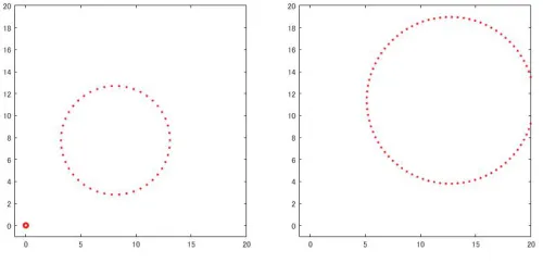
Figure 7: Examples of synthesized data. Left: S2 exists. Right: S2 does not exist. For the binary classification, we introduce the following labels:
z0= 1 if there exists a generator (b, d) in the persistence diagram such that b≤1 andd≥4. z1= 1 if S2 exists.
The class label of the data set is then given by XOR(z0, z1). By this construction, identi-fying z0 requires relatively smooth function in the area of long lifetimes, while classifying the existing ofz1 needs delicate control of the resolution around the diagonal.
4.2.2 SVM Results
SVMs are trained from persistence diagrams given by 100 data sets, and evaluated with 100 independent test data sets. As a positive definite kernel k, we choose the Gaussian kernel kGand the linear kernelkL(x, y) :=hx, yiR2. For a weight function w, we use the proposed functionwarc(x) = arctan(Cpers(x)p), the piecewise linear weighting functionwpers(x), and
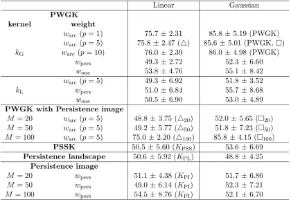
an unweighted function wone(x)≡1. The hyper-parameters (σ, C) in the PWGK and tin the PSSK are chosen by the 10-fold cross-validation, and the degree p in warc(x) is set as 1,5,10. For KPSS and KPL, while they originally consider only the inner product, we also apply the Gaussian kernels on RKHS following Equation (13). Since KPI can be seen as a discretization of the (kG, wpers)-linear kernel, we also construct another kernel of persistence image by replacing wpers with warc, which is considered as a discretization of the PWGK. In order to check whether the persistence image with warc is an appropriate discretization of the PWGK, we try several mesh size M = 20,50,100.
Linear Gaussian PWGK
kernel weight
warc (p= 1) 75.7±2.31 85.8±5.19 (PWGK) warc (p= 5) 75.8 ±2.47 (4) 85.6 ±5.01 (PWGK,) kG warc (p= 10) 76.0±2.39 86.0±4.98 (PWGK)
wpers 49.3±2.72 52.3 ±6.60 wone 53.8±4.76 55.1 ±8.42 warc (p= 5) 49.3±6.92 51.8 ±3.52
kL wpers 51.0±6.84 55.7 ±8.68
wone 50.5±6.90 53.0 ±4.89 PWGK with Persistence image
M = 20 warc (p= 5) 48.8±3.75 (420) 52.0 ±5.65 (20) M = 50 warc (p= 5) 49.2±5.77 (450) 51.8 ±7.23 (50) M = 100 warc (p= 5) 75.0 ±2.20 (4100) 85.8± 4.15 (100)
PSSK 50.5± 5.60 (KPSS) 53.6 ±6.69 Persistence landscape 50.6 ±5.92 (KPL) 48.8 ±4.25
Persistence image
M = 20 wpers 51.1±4.38 (KPI) 51.7 ±6.86 M = 50 wpers 49.0±6.14 (KPI) 52.3 ±7.21 M = 100 wpers 54.5±8.76 (KPI) 52.1 ±6.70
than the other methods (KPSS: 50%,KPL: 50%, andKPI: 55%). Although the (kG, wpers )-Gaussian kernel and the persistence image with the original weight wpers discount noisy generators, the classification rates are close the chance level. These unfavorable results must be caused by the difficulty in handling the local and global locations of generators simultaneously. While the result of the persistence image with a large mesh size is similar to that of the PWGK (e.g.,and100), a small mesh size gives bad approximation results (e.g.,and50). The reason is because a small mesh size makes rough pixels, andS2 itself and noisy generators are treated in some rough pixel. On the other hand, we remark that a large mesh size M needs much computational time.
We observe that the classification accuracies are not sensitive to p. Thus, in the rest of this paper, we set p = 5 because the assumption p > d+ 1 in Theorem 9 ensures the continuity in the kernel embedding of persistence diagrams and all data points are obtained from R3.
4.3 Analysis of Granular System
We apply the PWGK, the PSSK, the persistence landscape, and the persistence image to persistence diagrams obtained by experimental data in a granular packing system (Francois et al., 2013). In this example, a partially crystallized packing with 150,000 monosized beads (diameter = 1mm, polydispersity = 0.025mm) in a container is obtained by experiments, where the configuration of the beads is imaged by means of X-ray Computed Tomography. One of the fundamental interests in the study of granular packings is to understand the transition from random packings to crystallized packings. In particular, the maximum packing density φ∗ that random packings can attain is still a controversial issue (e.g., see Torquato et al. (2000)). Here, we apply the change point analysis to detectφ∗.
In oder to observe configurations of various densities, we divide the original full system into 35 cubical subsets containing approximately 4000 beads. The data are provided by the authors of the paper (Francois et al., 2013). The packing densities of the subsets range from φ= 0.590 to φ= 0.730. Saadatfar et al. (2017) computed a persistence diagram for each subset by taking the beads configuration as a finite subset in R3, and found that the persistence diagrams characterize different configurations in random packings (smallφ) and crystallized packings (largeφ). Hence, it is expected that the change point analysis applied to these persistence diagrams can detect the maximum packing density φ∗ as a transition from the random to crystallized packings.
Our strategy is to regard the maximum packing density as the change point and detect it from a collection D = {D` | ` = 1, . . . , n} (n = 35) of persistence diagrams made by
beads configurations of granular systems, where`is the index of the packing densities listed in the increasing order. As a statistical quantity for the change point detection, we use the kernel Fisher discriminant ratio (Harchaoui et al., 2009) defined by
KFDRn,`,γ(D) =
`(n−`) n
` nΣˆ1:`+
n−`
n Σˆ`+1:n+γI
−12
(ˆµ`+1:n−µˆ1:`)
HK
where the empirical mean element ˆµi:j and the empirical covariance operator ˆΣi:j with data
Di through Dj (i < j) are given by
ˆ µi:j =
1 j−i+ 1
j
X
`=i
K(·, D`),
ˆ Σi:j =
1 j−i+ 1
j
X
`=i
(K(·, D`)−µˆi:j)⊗(K(·, D`)−µˆi:j)
respectively, andγ is a regularization parameter (in this paper we setγ = 10−3). The index `achieving the maximum of KFDRn,`,γ(D) corresponds to the estimated change point. In
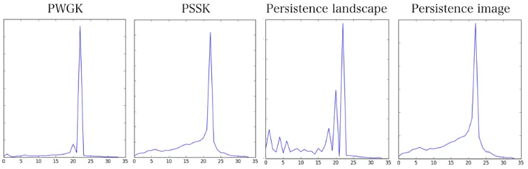
Figure 8, all the four methods detect ` = 23 as the sharp maximizer of the KFDR. This result indicates that the maximum packing density φ∗ exists in the interval [0.604,0.653] and supports the traditional observation φ∗≈0.636 (Anonymous, 1972).
Figure 8: The KFDR graphs of the PWGK, the PSSK, the persistence landscape, and the persistence image.
We also apply kernel principal component analysis (KPCA) to the same collection of the 35 persistence diagrams. Figure 9 shows the 2-dimensional KPCA plots where each blue cross (resp. red circle) indicates the persistence diagram of random packing (resp. crystallized packing). We can see clear two-cluster structure corresponding to two physical states.
4.4 Analysis of SiO2
Persistence landscape Persistence image PSSK
PWGK
Figure 9: The KPCA plots of the PWGK (contribution rate: 92.9%), the PSSK (99.7%), the persistence landscape (83.8%), and the persistence image (98.7%).
to prepare atomic configurations of SiO2 for a certain range of temperatures by molecular dynamics simulations, and then draw the temperature-enthalpy graph. The graph consists of two lines in high and low temperatures with slightly different slopes which correspond to the liquid and the glass states, respectively, and the glass transition temperature is conventionally estimated as an interval of the transient region combining these two lines (e.g., see Elliott (1990)). However, since the slopes of two lines are close to each other, determining the interval is a subtle problem. Usually only the rough estimate of the interval is available. Hence, we apply our framework of topological data analysis with kernels to detect the glass transition temperature.
Let {D` | ` = 1, . . . ,80} be a collection of the persistence diagrams made by atomic
configurations of SiO2 and sorted by the decreasing order of the temperature. The same data was used in the previous works by Hiraoka et al. (2016); Nakamura et al. (2015). The interval of the glass transition temperature T estimated by the conventional method explained above is 2000K≤T ≤3500K, which corresponds to 35≤`≤50.
In Figure 10, the KFDR plots show that the change point is estimated as `= 39 by the PWGK, ` = 33 by the PSSK, and ` = 33 by the persistence image. For the persistence landscape, we cannot obtain the KFDR or the KPCA results with reasonable computational time.
Persistence image PSSK
PWGK
Figure 11: The 2-dimensional and 3-dimensional KPCA plots of the PWGK (contribution rates for 2-dimension: 81.7%, 3-dimension: 92.1%), the PSSK (97.2%, 99.3%) and the persistence image (99.9%, 99.9%).
As we see from the 2-dimensional plots given by KPCA (Figure 11), the PWGK presents sharp change of the gradients between before (blue cross) and after (red circle) the change point determined by the KFDR. This matches with the analysis in physics that expects a sharp change of slope in the temperature-enthalpy plane. This strongly suggests that the glass transition occurs at the detected change point. On the other hand, in the results of PSSK and persistence images we cannot observe a sharp change of the gradients at the boundary of the estimated two phases. We also remark that clearer structures are observed in the 3-dimensional KPCA plots of the PWGK.
4.5 Protein Classification
Protein-Drug Hemoglobin
PWGK 100 88.90
MTF (nbd) 93.91 / (bd) 98.31 84.50
Table 2: CV classification rates (%) of SVMs with the PWGK and the MTF (cited from Cang et al. (2015)).
in persistence diagrams.17 We compare the performance between the PWGK and the MTF method under the same setting of the SVM reported in Cang et al. (2015).
The first task is a protein-drug binding problem, where the binding and non-binding of drug to the M2 channel protein of the influenza A virus is to be classified. For each of the two forms, 15 data were obtained by NMR experiments, and 10 data are used for training and the remaining for testing. We randomly generate 100 ways of partitions and calculate the average classification rates.
In the second problem, the taut and relaxed forms of hemoglobin are to be classified. For each form, 9 data were collected by the X-ray crystallography. We select one data from each class for testing and use the remaining for training. All the 81 combinations are performed to calculate the CV classification rates.
The results of the two problems are shown in Table 4.5. We can see that the PWGK achieves better performance than the MTF in both problems.
5. Conclusion and Discussions
One of the contributions of this paper is to introduce a kernel framework to topological data analysis with persistence diagrams. We applied the kernel embedding approach to vectorize the persistence diagrams, which enables us to utilize any standard kernel methods for data analysis. Another contribution is to propose a kernel specific to persistence diagrams, that is called persistence weighted Gaussian kernel (PWGK). As a significant advantage, our kernel enables one to control the effect of persistence in data analysis. We have also proven the stability property with respect to the distance in the Hilbert space. Furthermore, we have analyzed the synthesized and real data by using the proposed kernel. The change point detection, the principal component analysis, and the support vector machine derived meaningful results for the tasks. From the viewpoint of computations, our kernel can utilize an efficient approximation to compute the Gram matrix.
One of the main theoretical results of this paper is the bottleneck stability of the PWGK (Theorem 9). It is obtained by restricting the class of persistence diagrams to that obtained from ball model filtrations. The reason of this restriction is because the total persistence can be bounded from above independent of the persistence diagram. Thus, one direction to extend this work is to examine the boundedness condition about the total persistence of other persistence diagrams, for example obtained from Rips complexes or sub-level sets.
Another direction to extend this work is to generalize the class of weight functions. The reason of the choice ofwarcis mainly for the stability property, but in principle, we can apply any weight function to data analysis. Even if we do not concern about stability properties, which weight function is practically good for data analysis? Suppose generators close to the diagonal are sometimes seen as important features. Then, our statistical framework can treat such small generators as significant ones by a weight function which has large weight close to the diagonal, while other statistical methods for persistence diagrams always see small generators as noisy ones. In addition, the weight function becomes better when it is constructed to satisfy the assumption (W1) or (W2), which implies the stability property. Acknowledgement
Appendix A. Topological tools
This section summarizes some topological tools used in the paper. To study topological properties algebraically, simplicial complexes are often considered as basic objects. We start with a brief explanation of simplicial complexes, and gradually increase the generality from simplicial homology to singular and persistent homology. For more details, see Hatcher (2002).
A.1 Simplicial complex
We first introduce a combinatorial geometric model called simplicial complex to define homology. Let P = {1, . . . , n} be a finite set (not necessarily points in a metric space). A simplicial complex with the vertex set P is defined by a collection S of subsets in P satisfying the following properties:
1. {i} ∈S fori= 1, . . . , n, and 2. if σ∈S and τ ⊂σ, thenτ ∈S.
Each subsetσ withq+ 1 vertices is called aq-simplex. We denote the set of q-simplices by Sq. A subcollectionT ⊂S which also becomes a simplicial complex (with possibly less
vertices) is called a subcomplex of S.
We can visually deal with a simplicial complexSas a polyhedron by pasting simplices in S into a Euclidean space. The simplicial complex obtained in this way is called a geometric realization, and its polyhedron is denoted by |S|. In this context, the simplices with small q correspond to points (q = 0), edges (q= 1), triangles (q= 2), and tetrahedra (q = 3). Example 1 Figure 12 shows two polyhedra of simplicial complexes
S={{1},{2},{3},{1,2},{1,3},{2,3},{1,2,3}}, T ={{1},{2},{3},{1,2},{1,3},{2,3}}.
1 2
3
1 2
3
Figure 12: The polyhedra of the simplicial complexes S (left) andT (right).
A.2 Homology
A.2.1 Simplicial homology
The procedure to define homology is summarized as follows: