Operator-valued Kernels for Learning from Functional Response Data

Operator-valued Kernels for Learning from Functional

Response Data

Hachem Kadri [email protected]

Aix-Marseille Universit´e, LIF (UMR CNRS 7279) F-13288 Marseille Cedex 9, France

Emmanuel Duflos [email protected]

Ecole Centrale de Lille, CRIStAL (UMR CNRS 9189) 59650 Villeneuve d’Ascq, France

Philippe Preux [email protected]

Universit´e de Lille, CRIStAL (UMR CNRS 9189) 59650 Villeneuve d’Ascq, France

St´ephane Canu [email protected]

INSA de Rouen, LITIS (EA 4108) 76801, St Etienne du Rouvray, France

Alain Rakotomamonjy [email protected] Universit´e de Rouen, LITIS (EA 4108)

76801, St Etienne du Rouvray, France

Julien Audiffren [email protected]

ENS Cachan, CMLA (UMR CNRS 8536) 94235 Cachan Cedex, France

Editor:John Shawe-Taylor

Abstract

In this paper1 _{we consider the problems of supervised classification and regression in the} case where attributes and labels are functions: a data is represented by a set of functions, and the label is also a function. We focus on the use of reproducing kernel Hilbert space theory to learn from such functional data. Basic concepts and properties of kernel-based learning are extended to include the estimation of function-valued functions. In this setting, the representer theorem is restated, a set of rigorously defined infinite-dimensional operator-valued kernels that can be valuably applied when the data are functions is described, and a learning algorithm for nonlinear functional data analysis is introduced. The methodology is illustrated through speech and audio signal processing experiments.

Keywords: nonlinear functional data analysis, operator-valued kernels, function-valued reproducing kernel Hilbert spaces, audio signal processing

1. Introduction

In this paper, we consider the supervised learning problem in a functional setting: each attribute of a data is a function, and the label of each data is also a function. For the sake

of simplicity, one may imagine real functions, though the work presented here is much more general; one may also think about those functions as being defined over time, or space, though again, our work is not tied to such assumptions and is much more general. To this end, we extend the traditional scalar-valued attribute setting to a function-valued attribute setting.

This shift from scalars to functions is required by the simple fact that in many ap-plications, attributes are functions: functions may be one dimensional such as economic curves (variation of the price of “actions”), load curve of a server, a sound, etc., or two or higher dimensional (hyperspectral images, etc.). Due to the nature of signal acquisition, one may consider that in the end, a signal is always acquired in a discrete fashion, thus providing a real vector. However, with the resolution getting finer and finer in many sen-sors, the amount of discrete data is getting huge, and one may reasonably wonder whether a functional point of view may not be better than a vector point of view. Now, if we keep aside the application point of view, the study of functional attributes may simply come as an intellectual question which is interesting for its own sake.

From a mathematical point of view, the shift from scalar attributes to function attributes will come as a generalization from scalar-valued functions to function-valued functions, a.k.a.“operators”. Reproducing Kernel Hilbert Spaces (RKHS) has become a widespread tool to deal with the problem of learning a function mapping the set Rp to the set of real

numbersR. Here, we have to deal with RKHS of operators, that are functions that map a

function, belonging to a certain space of functions, to a function belonging to an other space of functions. This shift in terminology is accompanied with a dramatic shift in concepts, and technical difficulties that have to be properly handled.

Thisfunctional regression problem, orfunctional supervised learning, is a challenging re-search problem, from statistics to machine learning. Most previous work has focused on the discrete case: the multiple-response (finite and discrete) function estimation problem. In the machine learning literature, this problem is better known under the name of vector-valued function learning (Micchelli and Pontil, 2005a), while in the field of statistics, researchers prefer to use the term multiple output regression (Breiman and Friedman, 1997). One pos-sible solution is to approach the problem from a univariate point of view, that is, assuming only a single response variable output from the same set of explanatory variables. However it would be more efficient to take advantage of correlation between the response variables by considering all responses simultaneously. For further discussion of this point, we refer the reader to Hastie et al. (2001) and references therein. More recently, relevant works in this context concern regularized regression with a sequence of ordered response variables. Many variable selection and shrinkage methods for single response regression are extended to the multiple response data case and several algorithms following the corresponding so-lution paths are proposed (Turlach et al., 2005; Simila and Tikka, 2007; Hesterberg et al., 2008).

functions (Micchelli and Pontil, 2005a) and matrix-valued reproducing kernels (Micchelli and Pontil, 2005b; Reisert and Burkhardt, 2007) can be used as a theoretical framework to develop nonlinear multi-task learning methods.

A primary motivation for this paper is to build on these previous studies and provide a similar framework for addressing the general case where the output space is infinite di-mensional. In this setting, the output space is a space of functions and elements of this space are called functional response data. Functional responses are frequently encountered in the analysis of time-varying data when repeated measurements of a continuous response variable are taken over a small period of time (Faraway, 1997; Yao et al., 2005). The rela-tionships among the response data are difficult to explore when the number of responses is large, and hence one might be inclined to think that it could be helpful and more natural to consider the response as a smooth real function. Moreover, with the rapid development of accurate and sensitive instruments and thanks to the currently available large storage resources, data are now often collected in the form of curves or images. The statistical framework underlying the analysis of these data as a single function observation rather than a collection of individual observations is called functional data analysis (FDA) and was first introduced by Ramsay and Dalzell (1991).

It should be pointed out that in earlier studies a similar but less explicit statement of the functional approach was addressed in Dauxois et al. (1982), while the first discussion of what is meant by “functional data” appears to be by Ramsay (1982). Functional data analysis deals with the statistical description and modeling of random functions. For a wide range of statistical tools, ranging from exploratory and descriptive data analysis to linear models and multivariate techniques, a functional version has been recently developed. Reviews of theoretical concepts and prospective applications of functional data can be found in the two monographs by Ramsay and Silverman (2005, 2002). One of the most crucial questions related to this field is “What is the correct way to handle large data? Multivariate or Functional?” Answering this question requires better understanding of complex data structures and relationship among variables. Until now, arguments for and against the use of a functional data approach have been based on methodological considerations or experimental investigations (Ferraty and Vieu, 2003; Rice, 2004). However, we believe that without further improvements in theoretical issues and in algorithm design of functional approaches, exhaustive comparative studies will remain hard to conduct.

This motivates the general framework we develop in this paper. To the best of our knowledge, nonlinear methods for functional data is a topic that has not been sufficiently addressed in the FDA literature. Unlike previous studies on nonlinear supervised classifica-tion or real response regression of funcclassifica-tional data (Rossi and Villa, 2006; Ferraty and Vieu, 2004; Preda, 2007), this paper addresses the problem of learning tasks where the output variables are functions. From a machine learning point of view, the problem can be viewed as that of learning a function-valued function f :X −→ Y where X is the input space and

attributes with functional attributes in this paper. This point has been discussed in (Kadri et al., 2011b). To deal with non-linearity, we adopt a kernel-based approach and we design operator-valued kernels that perform the mapping between the two spaces of functions. Our main results demonstrate how basic concepts and properties of kernel-based learning known in the case of multivariate data can be restated for functional data.

Extending learning methods from multivariate to functional response data may lead to further progress in several practical problems of machine learning and applied statistics. To compare the proposed nonlinear functional approach with other multivariate or functional methods and to apply it in a real world setting, we are interested in the problems of speech inversion and sound recognition, which have attracted increasing attention in the speech processing community in the recent years (Mitra et al., 2010; Rabaoui et al., 2008). These problems can be cast as a supervised learning problem which include some components (pre-dictors or responses) that may be viewed as random curves. In this context, though some concepts on the use of RKHS for functional data similar to those presented in this work can be found in Lian (2007), the present paper provides a much more complete view of learning from functional data using kernel methods, with extended theoretical analysis and several additional experimental results.

This paper is a combined and expanded version of our previous conference papers (Kadri et al., 2010, 2011c). It gives the full justification, additional insights as well as new and comprehensive experiments that strengthen the results of these preliminary conference pa-pers. The outline of the paper is as follows. In Section 2, we discuss the connection between the two fields Functional Data Analysis and Machine Learning, and outline our main con-tributions. Section 3 defines the notation used throughout the paper. Section 4, describes the theory of reproducing kernel Hilbert spaces of function-valued functions and shows how vector-valued RKHS concepts can be extended to infinite-dimensional output spaces. In Section 5, we exhibit a class of operator-valued kernels that perform the mapping between two spaces of functions and discuss some ideas for understanding their associated feature maps. In Section 6, we provide a function-valued function estimation procedure based on inverting block operator kernel matrices, propose a learning algorithm that can handle func-tional data, and analyze theoretically its generalization properties. Finally in Section 7, we illustrate the performance of our approach through speech and audio processing experi-ments.

2. The Interplay of FDA and ML Research

0 0.1 0.2 0.3 0.4 0.5 0.6 0

0.5 1 1.5 2

seconds

Millivolts

EMG curves

0 0.1 0.2 0.3 0.4 0.5 0.6 −3

−2 −1 0 1 2 3

seconds

Meters/s

2

Lip acceleration curves

Figure 1: Electromyography (EMG) and lip acceleration curves. The left panel displays EMG recordings from a facial muscle that depresses the lower lip, the depressor labii inferior. The right panel shows the accelerations of the center of the lower lip of a speaker pronouncing the syllable “bob”, embedded in the phrase “Say bob again”, for 32 replications (Ramsay and Silverman, 2002, Chapter 10).

with data in infinite-dimensional spaces, it does not appear to be commonplace for machine learners. One possible reason for this lack of success is that the formal use of infinite di-mensional spaces for practical ML applications may seem unjustified; because in practice traditional measurement devices are limited in providing discrete and not functional data, and a machine learning algorithm can process only finitely represented objects. We believe that for applied machine learners it should be vital to know the full range of applicabil-ity of functional data analysis and infinite-dimensional data representations. But due to limitation of space we shall say only few words about the occurrence of functional data in real applications and about the real learning task lying behind this kind of approach. The reader is referred to Ramsay and Silverman (2002) for more details and references. Areas of application discussed and cited there include medical diagnosis, economics, meteorology, biomechanics, and education. For almost all these applications, the high-sampling rate of today’s acquisition devices makes it natural to directly handle functions/curves instead of discretized data. Classical multivariate statistical methods may be applied to such data, but they cannot take advantage of the additional information implied by the smoothness of the underlying functions. FDA methods can have beneficial effects in this direction by extract-ing additional information contained in the functions and their derivatives, not normally available through traditional methods (Levitin et al., 2007).

To get a better idea about the natural occurrence of functional data in ML tasks, Figure 1 depicts a functional data set introduced by Ramsay and Silverman (2002). The data set consists of 32 records of the movement of the center of the lower lip when a subject was repeatedly required to say the syllable “bob”, embedded in the sentence, “Say bob again” and the corresponding EMG activities of the primary muscle depressing the lower lip, the depressor labii inferior (DLI)2. The goal here is to study the dependence of the acceleration

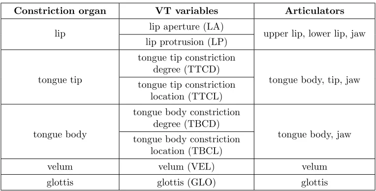
Figure 2: “Audio signal (top), tongue tip trajectory (middle), and jaw trajectory (bottom) for the utterance [­nOnO"nOnO]. The trajectories were measured by electromagnetic articulography (EMA) for coils on the tongue tip and the lower incisors. Each trajectory shows the displacement along the first principal component of the original two-dimensional trajectory in the midsagittal plane. The dashed curves show hypothetical continuations of the tongue tip trajectory towards and away from virtual targets during the closure intervals.” (Birkholz et al., 2010).

of the lower lip in speech on neural activity. EMG and lip accelerations curves can be well modeled by continuous functions of time that allow to capture functional dependencies and interactions between samples (feature values). Thus, we face a regression problem where both input and output data are functions. In much the same way, Figure 2 also shows a “natural” representation of data in terms of functions 3. It represents a speech signal used for acoustic-articulatory speech inversion and produced by a subject pronouncing a sequence of [­CVCV"CVCV] (C=consonant, V=vowel) by combining the vowel {/O/} with the consonant{/n/}. The articulatory trajectories are represented by the upper and lower solid curves that show the displacement of fleshpoints on the tongue tip and the jaw along the main movement direction of these points during the repeated opening and closing gestures. This example is from a recent study on the articulatory modeling of speech signals (Birkholz et al., 2010). The concept of articulatory gestures in the context of speech-to-articulatory inversion will be explained in more details in Section 7. As shown in the figure, the observed articulatory trajectories are typically modeled by smooth functions of time with periodicity properties and exponential or sigmoidal shape, and the goal of speech inversion is to predict and recover geometric data of the vocal tract from the speech information.

In both examples given above, response data clearly present a functional behavior that should be taken into account during the learning process. We think that handling these data as what they really are, that is functions, is a promising way to tackle prediction problems and design efficient ML systems for continuous data variables. Moreover, ML methods which

can handle functional features can open up plenty of new areas of application, where the flexibility of functional and infinite-dimensional spaces would allow to enable us to achieve significantly better performance while managing huge amounts of training data.

In the light of these observations, there is an interest in overcoming methodological and practical problems that hinder the wide adoption and use of functional methods built for infinite-dimensional data. Regarding the practical issue related to the application and im-plementation of infinite-dimensional spaces, a standard means of addressing it is to choose a functional space a priori with a known predefined set of basis functions in which the data will be mapped. This may include a preprocessing step, which consists in con-verting the discretized data into functional objects using interpolation or approximation techniques. Following this scheme, parametric FDA methods have emerged as a common approach to extend multivariate statistical analysis in functional and infinite-dimensional situations (Ramsay and Silverman, 2005). More recently, nonparametric FDA methods have received increasing attention because of their ability to avoid fixing a set of basis functions for the functional data beforehand (Ferraty and Vieu, 2006). These methods are based on the concept of metrics for modeling functional data. The reason for using a semi-metric rather than a semi-metric is that the coincidence axiom, namelyd(xi, xj) = 0⇔xi=xj,

may result in curves with very similar shapes being categorized as distant (not similar to each other). To define closeness between functions in terms of shape rather than location semi-metrics can be used. In this spirit, Ferraty and Vieu (2006) provided a semi-metric based methodology for nonparametric functional data analysis and argued that this can be a sufficiently general theoretical framework to tackle infinite-dimensional data without being “too heavy” in terms of computational time and implementation complexity.

Thus, although both parametric and nonparametric functional data analyses deal with infinite-dimensional data, they are computationally feasible and quite practical since the observed functional data are approximated in a basis of the function space with possibly finite number of elements. What we really need is the inner or semi-inner product of the basis elements and the representation of the functions with respect to that basis. We think that Machine Learning research can profit from exploring other representation formalisms that support the expressive power of functional data. Machine learning methods which can accommodate functional data should open up new possibilities for handling practical appli-cations for which the flexibility of infinite-dimensional spaces could be exploited to achieve performance benefits and accuracy gains. On the other hand, in the FDA field, there is clearly a need for further development of computationally efficient and understandable al-gorithms that can deliver near-optimal solutions for infinite-dimensional problems and that can handle a large number of features. The transition from infinite-dimensional statistics to efficient algorithmic design and implementation is of central importance to FDA methods in order to make them more practical and popular. In this sense, Machine Learning can have a profound impact on FDA research.

2002). Depending on the choice of the kernel function, the feature space can be infinite-dimensional. The kernel trick is used, allowing to work with finite Gram matrix of inner products between the possibly infinite-dimensional features which can be seen as functional data. This connection between kernel and FDA methods is clearer with the concept of ker-nel embedding of probability distributions, where, instead of (observed) single points, kerker-nel means are used to represent probability distributions (Smola et al., 2007; Sriperumbudur et al., 2010). The kernel mean corresponds to a mapping of a probability distribution in a feature space which is rich enough so that its expectation uniquely identifies the distri-bution. Thus, rather than relying on large collections of vector data, kernel-based learning can be adapted to probability distributions that are constructed to meaningfully represent the discrete data by the use of kernel means (Muandet et al., 2012). In some sense, this represents a similar design to FDA methods, where data are assumed to lie in a functional space even though they are acquired in a discrete manner. There are also other papers that deal with machine learning problems where covariates are probability distributions and discuss their relation with FDA (Poczos et al., 2012, 2013; Oliva et al., 2013). At that point, however, the connection between ML and FDA is admittedly weak and needs to be bolstered by the delivery of more powerful and flexible learning machines that are able to deal with functional data and infinite-dimensional spaces.

In the FDA field, linear models have been explored extensively. Nonlinear modeling of functional data is, however, a topic that has not been sufficiently investigated, especially when response data are functions. Reproducing kernels provide a powerful tool for solving learning problems with nonlinear models, but to date they have been used more to learn scalar-valued or vector-valued functions than function-valued functions. Consequently, ker-nels for functional response data and their associated function-valued reproducing kernel Hilbert spaces have remained mostly unknown and poorly studied. In this work, we aim to rectify this situation, and highlight areas of overlap between the two fields FDA and ML, particularly with regards to the applicability and relevance of the FDA paradigm cou-pled with machine learning techniques. Specifically, we provide a learning methodology for nonlinear FDA based on the theory of reproducing kernels. The main contributions are as follows:

• we introduce a set of rigorously defined operator-valued kernels suitable for functional response data, that can be valuably applied to model dependencies between samples and take into account the functional nature of the data, like the smoothness of the curves underlying the discrete observations,

• we propose an efficient algorithm for learning function-valued functions (operators) based on the spectral decomposition of block operator matrices,

• we study the generalization performance of our learned nonlinear FDA model using the notion of algorithmic stability,

3. Notations and Conventions

We start by some standard notations and definitions used all along the paper. Given a Hilbert space H, h·,·iH and k · kH refer to its inner product and norm, respectively.

Hn = H ×. . .× H

| {z }

ntimes

, n ∈ _N+, denotes the topological product of n spaces H. We denote by X = {x : Ωx −→ R} and Y = {y : Ωy −→ R} the separable Hilbert spaces of input

and output real-valued functions whose domains are Ωx and Ωy, respectively. In functional

data analysis domain, the space of functions is generally assumed to be the Hilbert space of equivalence classes of square integrable functions, denoted by L2. Thus, in the rest of the paper, we considerYto be the spaceL2(Ωy), where Ωy is a compact set. The vector space of

functions fromX intoYis denoted byYX _{endowed with the topology of uniform convergence} on compact subsets of X. We denote by C(X,Y) the vector space of continuous functions

from X to Y, by F ⊂ YX the Hilbert space of function-valued functionsF :X −→ Y, and

by L(Y) the set of bounded linear operators fromY toY.

We now fix the following conventions for bounded linear operators and block operator matrices.

Definition 1 (adjoint, self-adjoint, and positive operators) Let A∈ L(Y). Then:

(i) A∗, the adjoint operator of A, is the unique operator inL(Y) that satisfies

hAy, ziY =hy, A∗ziY , ∀y∈ Y,∀z∈ Y,

(ii) A is self-adjoint if A=A∗,

(iii) A is positive if it is self-adjoint and ∀y∈ Y, hAy, yiY ≥0 (we write A≥0),

(iv) A is larger or equal than B ∈ L(Y), if A−B is positive, i.e., ∀y ∈ Y, hAy, yiY ≥

hBy, yiY (we write A≥B).

Definition 2 (block operator matrix) Let n∈_N, let Yn_{=Y ×. . .× Y}

| {z }

ntimes

.

(i) A∈ L(Yn_{), given by}

A=



 

A11 . . . A1n ..

. ...

An1 . . . Ann 

 

where each Aij ∈ L(Y), i, j= 1, . . . , n, is called a block operator matrix,

(ii) the adjoint (or transpose) of A is the block operator matrix A∗ ∈ L(Yn_{) such that}

(A∗)ij = (Aji)∗,

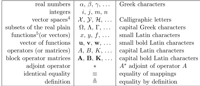
real numbers α,β,γ,. . . Greek characters integers i,j,m,n

vector spaces4 _{X,Y,H,. . . Calligraphic letters}

subsets of the real plain Ω, Λ, Γ,. . . capital Greek characters functions5(or vectors) x,y,f,. . . small Latin characters

vector of functions u,v,w,. . . small bold Latin characters operators (or matrices) A,B,K,. . . capital Latin characters block operator matrices A,B,K,. . . capital bold Latin characters

adjoint operator ∗ A∗ adjoint of operatorA

identical equality ≡ equality of mappings

definition , equality by definition

Table 1: Notations used in this paper.

Note that item (ii) in Definition 2 is obtained from the definition of adjoint operator. It is easy to see that ∀y ∈ Yn _{and ∀z ∈ Y}n_{; we have: hAy,zi}

Yn = P i,j

hA_ijyj, ziiY =

P

i,j

hyj, A∗ijziiY =P

i,j

hyj,(A∗)jiziiY =hy,A∗ziYn, where (A∗)_ji = (A_ij)∗.

To help the reader, notations frequently used in the paper are summarized in Table 1.

4. Reproducing Kernel Hilbert Spaces of Function-valued Functions

Hilbert spaces of scalar-valued functions with reproducing kernels were introduced and studied in Aronszajn (1950). Due to their crucial role in designing kernel-based learning methods, these spaces have received considerable attention over the last two decades (Shawe-Taylor and Cristanini, 2004; Sch¨olkopf and Smola, 2002). More recently, interest has grown in exploring reproducing Hilbert spaces of vector functions for learning vector-valued func-tions (Micchelli and Pontil, 2005a; Carmeli et al., 2006; Caponnetto et al., 2008; Carmeli et al., 2010; Zhang et al., 2012), even though the idea of extending the theory of Repro-ducing Kernel Hilbert Spaces from the scalar-valued case to the vector-valued one is not new and dates back to at least Schwartz (1964). For more details, see the review paper by ´Alvarez et al. (2012).

In the field of machine learning, Evgeniou et al. (2005) have shown how Hilbert spaces of vector-valued functions and matrix-valued reproducing kernels can be used in the context of multi-task learning, with the goal of learning many related regression or classification tasks simultaneously. Since this seminal work, it has been demonstrated that these kernels and their associated spaces are capable of solving various other learning problems such as multiple output learning (Baldassarre et al., 2012), manifold regularization (Minh and Sindhwani, 2011), structured output prediction (Brouard et al., 2011; Kadri et al., 2013a), multi-view learning (Minh et al., 2013; Kadri et al., 2013b) and network inference (Lim et al., 2013, 2015).

4. We also use the standard notations such asRnandL2.

In contrast to most of these previous works, here we are interested in the general case where the output space is a space of vectors with infinite dimension. This may be valuable from a variety of perspectives. Our main motivation is the supervised learning problem when output data are functions that could represent, for example, one-dimensional curves (this was mentioned as future work in Szedmak et al. 2006). One of the simplest ways to handle these data is to treat them as multivariate vectors. However this method does not consider any dependency of different values over subsequent time-points within the same functional datum and suffers when data dimension is very large. Therefore, we adopt a functional data analysis viewpoint (Zhao et al., 2004; Ramsay and Silverman, 2005; Ferraty and Vieu, 2006) in which multiple curves are viewed as functional realizations of a single function. It is important to note that matrix-valued kernels for infinite-dimensional output spaces, com-monly known as operator-valued kernels, have been considered in previous studies (Micchelli and Pontil, 2005a; Caponnetto et al., 2008; Carmeli et al., 2006, 2010); however, they have been only studied in a theoretical perspective. Clearly, further investigations are needed to illustrate the practical benefits of the use of operator-valued kernels, which is the main focus of this work.

We now describe how RKHS theory can be extended from real or vector to functional response data. In particular, we focus on reproducing kernel Hilbert spaces whose ele-ments are function-valued functions (or operators) and we demonstrate how basic proper-ties of real-valued RKHS can be restated in the functional case, if appropriate conditions are satisfied. Extension to the functional case is not so obvious and requires tools from functional analysis (Rudin, 1991). Spaces of operators whose range is infinite-dimensional can exhibit unusual behavior, and standard topological properties may not be preserved in the infinite-dimensional case because of functional analysis subtleties. So, additional restrictions imposed on these spaces are needed for extending the theory of RKHS to-wards infinite-dimensional output spaces. Following Carmeli et al. (2010), we mainly focus on separable Hilbert spaces with reproducing operator-valued kernels whose elements are continuous functions. This is a sufficient condition to avoid topological and measurability problems encountered with this extension. For more details about vector or function-valued RKHS of measurable and continuous functions, see Carmeli et al. (2006, Sections 3 and 5). Note that the framework developed in this section should be valid for any type of input data (vectors, functions, or structures). In this paper, however, we consider the case where both input and output data are functions.

Definition 3 (Operator-valued kernel)

An L(Y)-valued kernel K on X2 _{is a function K(·,·) :X × X −→ L(Y);}

(i) K is Hermitian if ∀x, z ∈ X, K(w, z) = K(z, w)∗, (where the superscript * denotes the adjoint operator),

(ii) K is nonnegative on X if it is Hermitian and for every natural number r and all

{(wi, ui)i=1,...,r} ∈ X × Y, the matrix with ij-th entry hK(wi, wj)ui, ujiY is

nonnega-tive (posinonnega-tive-definite).

Definition 4 (Block operator kernel matrix)

corresponding block operator kernel matrix is the matrixK∈ L(Yn_{) with entries} Kij =K(wi, wj).

The block operator kernel matrix is simply the kernel matrix associated to an operator-valued kernel. Since the kernel outputs an operator, the kernel matrix is in this case a block matrix where each block is an operator in L(Y). It is easy to see that an operator-valued kernel K is nonnegative if and only if the associated block operator kernel matrix K is positive.

Definition 5 (Function-valued RKHS)

A Hilbert space F of functions from X to Y is called a reproducing kernel Hilbert space if there is a nonnegativeL(Y)-valued kernel K onX2 _{such that:}

(i) the functionz7−→K(w, z)g belongs toF,∀z, w ∈ X and g∈ Y,

(ii) for everyF ∈ F, w∈ X andg∈ Y, hF, K(w,·)giF =hF(w), giY.

On account of (ii), the kernel is called the reproducing kernel of F. In Carmeli et al. (2006, Section 5), the authors provided a characterization of RKHS with operator-valued kernels whose functions are continuous and proved that F is a subspace of C(X,Y), the vector space of continuous functions from X toY, if and only if the reproducing kernel K

is locally bounded and separately continuous. Such a kernel is qualified as Mercer (Carmeli et al., 2010). In the following, we will only consider separable RKHS F ⊂ C(X,Y).

Theorem 1 (Uniqueness of the reproducing operator-valued kernel)

If a Hilbert space F of functions from X to Y admits a reproducing kernel, then the reproducing kernel K is uniquely determined by the Hilbert space F.

Proof: LetK be a reproducing kernel ofF. Suppose that there exists another reproducing kernelK0ofF. Then, for all{w, w0_{} ∈ X and{h, g} ∈ Y, applying the reproducing property} forK andK0 we get

hK0(w0,·)h, K(w,·)giF =hK0(w0, w)h, giY, (1) we have also

hK0_(w0_{,·)h, K(w,·)gi}

F = hK(w,·)g, K0(w0,·)hiF = hK(w, w0)g, hiY

= hg, K(w, w0)∗hiY = hg, K(w0, w)hiY. (2)

(1) and (2) ⇒K(w, w0)≡K0(w, w0), ∀w, w0 ∈ X.

Theorem 2 (Bijection between function-valued RKHS and operator-valued kernel)

A L(Y)-valued Mercer kernel K onX2 _{is the reproducing kernel of some Hilbert space F,} if and only if it is nonnegative.

We give a proof of this theorem by extending the scalar-valued case Y =R in Aronszajn

(1950) to the domain of functional data analysis domain whereY isL2(Ωy).6 The proof is

performed in two steps. The necessity is an immediate result from the reproducing property. For the sufficiency, the outline of the proof is as follows: we assumeF0 to be the space of

all Y-valued functions F of the form F(·) = Pn

i=1K(wi,·)ui, where wi ∈ X and ui ∈ Y,

with the following inner product hF(·), G(·)i_F

0 =

Pn

i=1

Pm

j=1hK(wi, zj)ui, vjiY defined for any G(·) = Pm

j=1K(zj,·)vj with zj ∈ X and vj ∈ Y. We show that (F0,h·,·iF0) is a

pre-Hilbert space. Then we complete this pre-pre-Hilbert space via Cauchy sequences{Fn(·)} ⊂ F0

to construct the Hilbert space F of Y-valued functions. Finally, we conclude that F is a reproducing kernel Hilbert space, since F is a real inner product space that is complete under the normk · kF defined bykF(·)kF = lim

n→∞kFn(·)kF0, and has K(·,·) as reproducing kernel.

Proof: Necessity. Let K be the reproducing kernel of a Hilbert space F. Using the reproducing property of the kernel K we obtain for any {w_i, wj} ∈ X and {ui, uj} ∈ Y

n X

i,j=1

hK(wi, wj)ui, ujiY = n X

i,j=1

hK(wi,·)ui, K(wj,·)ujiF

=h

n X

i=1

K(wi,·)ui, n X

i=1

K(wi,·)uiiF =k

n X

i=1

K(wi,·)uik2F ≥ 0.

Sufficiency. Let F₀ ⊂ YX _{be the space of all Y-valued functions F of the form F(·) =}

n P

i=1

K(wi,·)ui, where wi ∈ X and ui ∈ Y,i= 1, . . . , n. We define the inner product of the

functions F(·) =

n P

i=1

K(wi,·)ui and G(·) = m P

j=1

K(zj,·)vj from F0 as follows

hF(·), G(·)iF0 =h n X

i=1

K(wi,·)ui, m X

j=1

K(zj,·)vjiF0 = n X i=1 m X j=1

hK(wi, zj)ui, vjiY.

hF(·), G(·)iF0 is a symmetric bilinear form onF0 and due to the positivity of the kernelK,

kF(·)k defined by

kF(·)k=phF(·), F(·)iF0

is a quasi-norm in F0. The reproducing property in F0 is verified with the kernel K. In

fact, if F ∈ F₀ then

F(·) =

n X

i=1

K(wi,·)ui,

and ∀(w, u)∈ X × Y,

hF, K(w,·)uiF0 =h n X

i=1

K(wi,·)ui, K(w,·)uiF0 =h n X

i=1

K(wi, w)ui, uiY =hF(w), uiY.

Moreover using the Cauchy-Schwartz inequality, we have: ∀ (w, u)∈ X × Y,

hF(w), uiY =hF(·), K(w,·)uiF0 ≤ kF(·)kF0kK(w,·)ukF0.

Thus, ifkFkF0 = 0, thenhF(w), uiY = 0 for anywandu, and henceF ≡0. Thus (F0,h., .iF0)

is a pre-Hilbert space. This pre-Hilbert space is in general not complete, but it can be com-pleted via Cauchy sequences to build the Y-valued Hilbert spaceF which hasK as repro-ducing kernel, which concludes the proof. The completion ofF0 is given in Appendix A (we

refer the reader to the monograph by Rudin, 1991, for more details about completeness and

the general theory of topological vector spaces).

We now give an example of a function-valued RKHS and its operator-valued kernel. This example serves to illustrate how these spaces and their associated kernels generalize the standard scalar-valued case or the vector-valued one to functional and infinite-dimensional output data. Thus, we first report an example of a scalar-valued RKHS and the corre-sponding scalar-valued kernel. We then extend this example to the case of vector-valued Hilbert spaces with matrix-valued kernels, and finally to function-valued RKHS where the output space is infinite dimensional. For the sake of simplicity, the input space X in these examples is assumed to be a subset ofR.

Example 1 (Scalar-valued RKHS and its scalar-valued kernel; see Canu et al. (2003)) Let F be the space defined as follows:

 



F =

f : [0,1]−→_Rabsolutely continuous, ∃f0∈L2([0,1]), f(x) =

Z x

0

f0(z)dz ,

hf₁, f2iH=hf10, f20iL2_([0,1]).

F is the Sobolev space of degree 1, also called the Cameron-Martin space, and is a scalar-valued RKHS of functionsf : [0,1]−→_Rwith the scalar-valued reproducing kernelk(x, z) =

min(x, z),∀x, z ∈ X = [0,1].

Example 2 (Vector-valued RKHS and its matrix-valued kernel)

Let X = [0,1] andY =Rn. Consider the matrix-valued kernelK defined by:

K(x, z) =

diag(x) if x≤z,

diag(z) otherwise, (3)

where, ∀a∈_R,diag(a)is then×ndiagonal matrix with diagonal entries equal toa. LetM

be the space of vector-valued functions fromX ontoRnwhose normkgk2M=

n X

i=1 Z

X

[g(x)]2_idx

The matrix-valued mappingKis the reproducing kernel of the vector-valued RKHSF defined as follows:

 



F =f : [0,1]−→_Rn, ∃f0= df(x)

dx ∈ M,[f(x)]i=

Z x

0

[f0(z)]idz,∀i= 1, . . . , n ,

hf1, f2iF =hf10, f20iM.

Indeed,K is nonnegative and we have, ∀x∈ X, y∈_Rn _{andf ∈ F,}

hf, K(x,·)yiF =hf0,[K(x,·)y]0iM

= n X i=1 Z 1 0

[f0(z)]i[K(x, z)y]0idz

= n X i=1 Z x 0

[f0(z)]iyidz (dK(x, z)/dz =diag(1) if z≤x, and =diag(0) otherwise)

=

n X

i=1

[f(x)]iyidz = hf(x), yiRn.

Example 3 (Function-valued RKHS and its operator-valued kernel)

Here we extend Example 2 to the case where the output space is infinite dimensional. Let X = [0,1] and Y = L2(Ω) the space of square integrable functions on a compact set

Ω⊂_R. We denote by M the space of L2(Ω)-valued functions on X whose norm kgk2

M =

Z

Ω Z

X

[g(x)(t)]2dxdt is finite.

Let (F;h·,·iF) be the space of functions from X toL2(Ω)such that:

 



F=f, ∃f0 = df(x)

dx ∈ M, f(x) =

Z x

0

f0(z)dz ,

hf1, f2iF =hf10, f20iM.

F is a function-valued RKHS with the operator-valued kernel K(x, z) =Mϕ(x,z). Mϕ is the multiplication operator associated with the function ϕ where ϕ(x, z) is equal to x if x ≤ z

and z otherwise. Since ϕ is a positive-definite function, K is Hermitian and nonnegative. Indeed,

hK(z, x)∗y, wiY =hy, K(z, x)wiY =

Z 1 0

ϕ(z, x)w(t)y(t)dt=

Z 1 0

ϕ(x, z)y(t)z(t)dt

=hK(x, z)y, wiY,

and

X

i,j

hK(xi, xj)yi, yjiY =

X

i,j Z 1

0

ϕ(xi, xj)yi(t)yj(t)dt

=

Z 1 0

X

i,j

Now we show that the reproducing property holds for anyf ∈ F,y ∈L2(Ω) andx∈ X:

hf, K(x,·)yiF =hf0,[K(x,·)y]0iM

=

Z

Ω Z 1

0

[f0(z)](t)[K(x, z)y]0(t)dzdt

kern.def

=

Z

Ω Z x

0

[f0(z)](t)y(t)dzdt=

Z

Ω

[f(x)](t)y(t)dt

=hf(x), yi_L2_(Ω).

Theorem 2 states that it is possible to construct a pre-Hilbert space of operators from a nonnegative operator-valued kernel and with some additional assumptions it can be com-pleted to obtain a function-valued reproducing kernel Hilbert space. Therefore, it is impor-tant to consider the problem of constructing nonnegative operator-valued kernels. This is the focus of the next section.

5. Operator-valued Kernels for Functional Data

Reproducing kernels play an important role in statistical learning theory and functional estimation. Scalar-valued kernels are widely used to design nonlinear learning methods which have been successfully applied in several machine learning applications (Sch¨olkopf and Smola, 2002; Shawe-Taylor and Cristanini, 2004). Moreover, their extension to matrix-valued kernels has helped to bring additional improvements in learning vector-matrix-valued func-tions (Micchelli and Pontil, 2005a; Reisert and Burkhardt, 2007; Caponnetto and De Vito, 2006). The most common and most successful applications of matrix-valued kernel methods are in multi-task learning (Evgeniou et al., 2005; Micchelli and Pontil, 2005b), even though some successful applications also exist in other areas, such as image colorization (Minh et al., 2010), link prediction (Brouard et al., 2011) and network inference (Lim et al., 2015). A ba-sic, albeit not obvious, question which is always present with reproducing kernels concerns how to build these kernels and what is the optimal kernel choice. This question has been studied extensively for scalar-valued kernels, however it has not been investigated enough in the matrix-valued case. In the context of multi-task learning, matrix-valued kernels are constructed from scalar-valued kernels which are carried over to the vector-valued setting by a positive definite matrix (Micchelli and Pontil, 2005b; Caponnetto et al., 2008).

In this section we consider the problem from a more general point of view. We are interested in the construction of operator-valued kernels, generalization of matrix-valued kernels in infinite dimensional spaces, that perform the mapping between two spaces of functions and which are suitable for functional response data. Our motivation is to build operator-valued kernels that are capable of giving rise to nonlinear FDA methods. It is worth recalling that previous studies have provided examples of operator-valued kernels with infinite-dimensional output spaces (Micchelli and Pontil, 2005a; Caponnetto et al., 2008; Carmeli et al., 2010); however, they did not focus either on building methodological connections with the area of FDA, or on the practical impact of such kernels on real-world applications.

design of such kernels will doubtless prove difficult, but it is necessary to develop reliable nonlinear FDA methods. Most FDA methods in the literature are based on linear para-metric models. Extending these methods to nonlinear contexts should render them more powerful and efficient. Our line of attack is to construct operator-valued kernels from op-erators already used to build linear FDA models, particularly those involved in functional response models. Thus, it is important to begin by looking at these models.

5.1 Linear Functional Response Models

FDA is an extension of multivariate data analysis suitable when data are functions. In this framework, a data is a single function observation rather than a collection of observations. It is true that the data measurement process often provides a vector rather than a function, but the vector is a discretization of a real attribute which is a function. Hence, a functional datum i is acquired as a set of discrete measured values, yi1, . . . , yip; the first task in

parametric (linear) FDA methods is to convert these values to a function yi with values

yi(t) computable for any desired argument value t. If the discrete values are assumed to be

noiseless, then the process is interpolation; but if they have some observational error, then the conversion from discrete data to functions is a regression task (e.g., smoothing) (Ramsay and Silverman, 2005).

A functional data model takes the form yi=f(xi) +i where one or more of the

compo-nentsyi,xi and i are functions. Three subcategories of such models can be distinguished:

predictorsxi are functions and responsesyi are scalars; predictors are scalars and responses

are functions; both predictors and responses are functions. In the latter case, which is the context we face, the functionf is a compact operator between two infinite-dimensional Hilbert spaces. Most previous works on this model suppose that the relation between func-tional responses and predictors is linear; for more details, see Ramsay and Silverman (2005) and references therein.

For functional input and output data, the functional linear model commonly found in the literature is an extension of the multivariate linear one and has the following form:

y(t) =α(t) +β(t)x(t) +(t), (4)

where α and β are the functional parameters of the model (Ramsay and Silverman, 2005, Chapter 14). This model is known as the “concurrent model” where “concurrent” means thaty(t) only depends onx att. The concurrent model is similar to the varying coefficient model proposed by Hastie and Tibshirani (1993) to deal with the case where the parameter

β of a multivariate regression model can vary over time. A main limitation of this model is that the responsey and the covariatexare both functions of the same argumentt, and the influence of a covariate on the response is concurrent or point-wise in the sense thatx only influences y(t) through its value x(t) at time t. To overcome this restriction, an extended linear model in which the influence of a covariatex can involve a range of argument values

x(s) was proposed; it takes the following form:

y(t) =α(t) +

Z

x(s)β(s, t)ds+(t), (5)

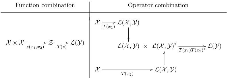
Function combination Operator combination

X × X

z(x1,x2) //Z T(z) //L(Y)

X

T(x1)//L(X,Y)

L(X,Y) × L(X,Y)∗

T(x1)T(x2)∗

//L(Y)

X

T(x2) //L(X,Y)

OO

Figure 3: Illustration of building an operator-valued kernel fromX ×X toL(Y) using a com-bination of functions or a comcom-bination of operators. (left) The operator-valued kernel is constructed by combining two functions (x1 and x2) and by applying a

positiveL(Y)-valued mappingT to the combination. (right) the operator-valued kernel is generated by combining two operators (T(x1) andT(x2)∗) built from an

L(X,Y)-valued mappingT.

2005, Chapter 16). Estimation of the parameter function β(·,·) is an inverse problem and requires regularization. Regularization can be implemented in a variety of ways, for example by penalized splines (James, 2002) or by truncation of series expansions (M¨uller, 2005). A review of functional response models can be found in Chiou et al. (2004).

The operators involved in the functional data models described above are the multi-plication operator (Equation 4) and the integral operator (Equation 5). We think that operator-valued kernels constructed using these operators could be a valid alternative to extend linear FDA methods to nonlinear settings. In Subsection 5.4 we provide examples of multiplication and integral operator-valued kernels. Before that, we identify building schemes that can be common to many operator-valued kernels and applied to functional data.

5.2 Operator-valued Kernel Building Schemes

In our context, constructing an operator-valued kernel turns out to build an operator that maps a couple of functions to a function: in X × X → L(Y) from two functions x1 and

x2 in X. This can be performed in one of two ways: either combining the two functions

x1 and x2 into a variable z ∈ Z and then adding an operator function T : Z −→ L(Y)

that performs the mapping from space Z toL(Y), or building an L(X,Y)-valued function

T, where L(X,Y) is the set of bounded operators from X to Y, and then combining the resulting operators T(x1) and T(x2) to obtain the operator in L(Y). In the latter case, a

natural way to combineT(x1) andT(x2) is to use the composition operation and the kernel

K(x1, x2) will be equal toT(x1)T(x2)∗. Figure 3 describes the construction of an

operator-valued kernel function using the two schemes which are based on combining functions (x1

and x2) or operators (T(x1) andT(x2)), respectively. Note that separable operator-valued

a scalar-valued kernel function for the input space alone and an operator that encodes the interactions between the outputs, are a particular case of the function combination building scheme, when we takeZ as the set of real numbersRand the scalar-valued kernel

as combination function. In contrast, the operator combination scheme is particularly amenable to the design of nonseparable operator-valued kernels. This scheme was already used in various problems of operator theory, system theory and interpolation (Alpay et al., 1997; Dym, 1989).

To build an operator-valued kernel and then construct a function-valued reproducing kernel Hilbert space, the operator T is of crucial importance. Choosing T presents two major difficulties. Computing the adjoint operator is not always easy to do, and then, not all operators verify the Hermitian condition of the kernel. On the other hand, since the kernel must be nonnegative, we suggest to construct operator-valued kernels from positive definite scalar-valued kernels which can be the reproducing kernels of real-valued Hilbert spaces. In this case, the reproducing property of the operator-valued kernel allows us to compute an inner product in a space of operators by an inner product in a space of functions which can be, in turn, computed using the scalar-valued kernel. The operator-valued kernel allows the mapping between a space of functions and a space of operators, while the scalar one establishes the link between the space of functions and the space of measured values. It is also useful to define combinations of nonnegative operator-valued kernels that allow to build a new nonnegative one.

5.3 Combinations of Operator-valued Kernels

We have shown in Section 4 that there is a bijection between nonnegative operator-valued kernels and function-valued reproducing kernel Hilbert spaces. So, as in the scalar case, it will be helpful to characterize algebraic transformations, like sum and product, that preserve the nonnegativity of operator-valued kernels. Theorem 3 stated below gives some building rules to obtain a positive operator-valued kernel from combinations of positive existing ones. Similar results for the case of matrix-valued kernels can be found in Reisert and Burkhardt (2007), and for a more general context we refer the reader to Caponnetto et al. (2008) and Carmeli et al. (2010). In our setting, assuming H and G be two nonnegative kernels constructed as described in the previous subsection, we are interested in constructing a nonnegative kernelK fromH and G.

Theorem 3 Let H:X × X −→ L(Y) andG:X × X −→ L(Y) two nonnegative operator-valued kernels

(i) K≡H+G is a nonnegative kernel,

(ii) if H(w, z)G(w, z) = G(w, z)H(w, z), ∀w, z ∈ X, then K ≡ HG is a nonnegative kernel,

(iii) K≡T HT∗ is a nonnegative kernel for any L(Y)-valued function T(·).

Proof: Obviously (i) follows from the linearity of the inner product. (ii) can be proved by showing that the “element-wise” multiplication of two positive block operator matrices can be positive (see below). For the proof of (iii), we observe that

and

X

i,j

hK(wi, wj)ui, uji= X

i,j

hT(wj)H(wi, wj)T(wi)∗ui, uji

=X

i,j

hH(wi, wj)T(wi)∗ui, T(wj)∗uji,

which implies the nonnegativity of the kernel K sinceH is nonnegative.

To prove (ii), i.e., the kernel K ≡ HG is nonnegative in the case where H and G are nonnegative kernels such thatH(w, z)G(w, z) =G(w, z)H(w, z),∀w, z∈ X, we show below that the block operator matrixKassociated to the operator-valued kernelK for a given set

{wi}, i= 1, . . . , n with n∈N, is positive. By construction, we have K =H◦Gwhere H

and G are the block operator kernel matrices corresponding to the kernels H and G, and ‘◦’ denotes the “element-wise” multiplication defined by (H◦G)ij = H(wi, wj)G(wi, wj). K,Hand Gare all in∈ L(Yn_).

Since the kernels H and G are Hermitian andHG=GH, it is easy to see that

(K∗)ij = (Kji)∗=K(wj, wi)∗ = H(wj, wi)G(wj, wi) ∗

=G(wj, wi)∗H(wj, wi)∗

=G(wi, wj)H(wi, wj) =H(wi, wj)G(wi, wj)

=Kij.

Thus,K is self-adjoint. It remains, then, to prove that hKu,ui ≥ 0,∀u ∈ Yn_{, in order to}

show the positivity ofK.

The “element-wise” multiplication can be rewritten as a tensor product. Indeed, we have

K=H◦G=L∗(H⊗G)L,

where L : Yn _{−→ Y}n_{⊗ Y}n _{is the mapping defined by Le}

i = ei⊗ei for an orthonormal basis {ei} of the separable Hilbert space Yn, and H⊗G is the tensor product defined by (H⊗G)(u⊗v) =Hu⊗Gv,∀u,v∈ Yn_{. To see this, note that}

hL∗(H⊗G)Lei,eji=h(H⊗G)Lei,Leji=h(H⊗G)(ei⊗ei),ej⊗eji =hHei⊗Gei,ej⊗eji=hHei,ejihGei,eji

=HijGij =h(H◦G)ei,eji.

Now sinceH and Gare positive, we have

hKu,ui=hL∗(H⊗G)Lu,ui=hL∗(H12H 1

2 ⊗G

1

2G

1

2)Lu,ui

=hL∗(H12 ⊗G 1

2)(H

1

2 ⊗G

1

2)Lu,ui=h(H

1

2 ⊗G

1

2)Lu,(H

1

2 ⊗G

1

2)∗Lui

=h(H12 ⊗G 1

2)Lu,(H

1

2 ⊗G

1

2)Lui=k(H

1

2 ⊗G

1

2)Luk2≥0.

This concludes the proof.

5.4 Examples of Nonnegative Operator-valued Kernels

We provide here examples of operator-valued kernels for functional response data. All these examples deal with operator-valued kernels constructed following the schemes described above and assuming that Y is an infinite-dimensional function space. Motivated by build-ing kernels suitable for functional data, the first two examples deal with operator-valued kernels constructed from the multiplication and the integral self-adjoint operators in the case where Y is the Hilbert space L2(Ωy) of square integrable functions on Ωy endowed

with the inner product hφ, ψi = R

Ωyφ(t)ψ(t)dt. We think that these kernels represent an interesting alternative to extend linear functional models to nonlinear settings. The third example based on the composition operator shows how to build such kernels from non self-adjoint operators (this may be relevant when the functional linear model is based on a non self-adjoint operator). It also illustrates the kernel combination defined in Theorem 3(iii).

1. Multiplication operator:

In Kadri et al. (2010), the authors attempted to extend the widely used Gaussian kernel to functional data domain using a multiplication operator and assuming that input and output data belong to the same space of functions. Here we consider a slightly different setting, where the input space X can be different from the output space Y.

A multiplication operator onY is defined as follows:

Th : Y −→ Y

y 7−→ T_yh ; T_yh(t),h(t)y(t).

The operator-valued kernelK(·,·) is the following:

K: X × X −→ L(Y)

x1, x2 7−→ kx(x1, x2)Tky,

wherekx(·,·) is a positive definite scalar-valued kernel andky a positive real function.

It is easy to see that hTh_{x, yi = hx, T}h_{yi, then T}h _{is a self-adjoint operator. Thus}

K(x2, x1)∗ =K(x2, x1) and K is Hermitian sinceK(x1, x2) =K(x2, x1).

Moreover, we have

X

i,j

hK(xi, xj)yi, yjiY =

X

i,j

kx(xi, xj)hky(·)yi(·), yj(·)iY

=X

i,j

kx(xi, xj) Z

ky(t)yi(t)yj(t)dt= Z

X

i,j

yi(t)[kx(xi, xj)ky(t)]yj(t)dt≥0,

since the product of two positive-definite scalar-valued kernels is also positive-definite. ThereforeK is a nonnegative operator-valued kernel.

2. Hilbert-Schmidt integral operator:

A Hilbert-Schmidt integral operator onY associated with a kernelh(·,·) is defined as follows:

Th : Y −→ Y

In this case, an operator-valued kernelK is a Hilbert-Schmidt integral operator asso-ciated with positive definite scalar-valued kernelskxandky, and it takes the following

form:

K(x1, x2)[·] : Y −→ Y

f 7−→ g

whereg(t) =kx(x1, x2) Z

ky(s, t)f(s)ds.

The Hilbert-Schmidt integral operator is self-adjoint ifky is Hermitian. This condition

is verified and then it is easy to check that K is also Hermitian. K is nonnegative since

X

i,j

hK(xi, xj)yi, yjiY =

Z Z X

i,j

yi(s)[kx(xi, xj)ky(s, t)]yj(t)dsdt,

which is positive because of the positive-definiteness of the scalar-valued kernels kx

and ky.

3. Composition operator:

Let ϕbe an analytic map. The composition operator associated withϕ is the linear map:

Cϕ :f 7−→f ◦ϕ

First, we look for an expression of the adjoint of the composition operatorCϕ acting

onY in the case whereYis a scalar-valued RKHS of functions on Ωyandϕan analytic

map of Ωy into itself. For anyf in the spaceY associated with the real kernel k,

hf, C∗

ϕkt(·)i = hCϕf, kti = hf◦ϕ, kti

= f(ϕ(t)) = hf, k_ϕ(t)i.

This is true for any f ∈ Y and then C_ϕ∗kt = kϕ(t). In a similar way, Cϕ∗f can be

computed at each point of the function f:

(C_ϕ∗f)(t) =hC_ϕ∗f, kti=hf, Cϕkti=hf, kt◦ϕi

Once we have expressed the adjoint of a composition operator in a reproducing kernel Hilbert space, we consider the following operator-valued kernel:

K : X × X −→ L(Y)

x1, x2 7−→ Cψ(x1)C_ψ∗_(x2)

whereψ(x1) andψ(x2) are maps of Ωy into itself. It is easy to see that the kernelK is

5.5 Multiple Functional Data and Kernel Feature Map

Until now, we discussed operator-valued kernels and their corresponding RKHS from the perspective of extending Aronszajn (1950) pioneering work from scalar-valued or vector-valued cases to the function-vector-valued case. However, it is also interesting to explore these kernels from a feature space point of view (Sch¨olkopf et al., 1999; Caponnetto et al., 2008). In this subsection, we provide some ideas targeted at advancing the understanding of feature spaces associated with operator-valued kernels and we show how these kernels can design more suitable feature maps than those associated with scalar-valued kernels, especially when input data are infinite dimensional objects like curves. To explore the potential of adopting an operator-valued kernel feature space approach, we consider a supervised learning problem with multiple functional data where each observation is composed of more than one functional variable (Kadri et al., 2011b,c). Working with multiple functions allows to deal in a natural way with a lot of applications. There are many practical situations where a number of potential functional covariates are available to explain a response variable. For example, in audio and speech processing where signals are converted into different functional features providing information about their temporal, spectral and cepstral characteristics, or in meteorology where the interaction effects between various continuous variables (such as temperature, precipitation, and winds) is of particular interest.

Similar to the scalar case, operator-valued kernels provide an elegant way of dealing with nonlinear algorithms by reducing them to linear ones in some feature space F nonlinearly related to input space. A feature map associated with an operator-valued kernel K is a continuous function

Φ :X × Y −→ L(X,Y),

such that for every x1, x2∈ X and y1, y2∈ Y

hK(x1, x2)y1, y2iY =hΦ(x1, y1),Φ(x2, y2)iL(X,Y),

where L(X,Y) is the set of linear mappings from X intoY. By virtue of this property, Φ is called afeature map associated with K. Furthermore, from the reproducing property, it follows that in particular

hK(x1,·)y1, K(x2,·)y2iF =hK(x1, x2)y1, y2iY,

which means that any operator-valued kernel admits a feature map representation Φ with a feature spaceF ⊂ L(X,Y) defined by Φ(x1, y1) = K(x1,·)y1, and corresponds to an inner

product in another space.

From this feature map perspective, we study the geometry of a feature space associated with an operator-valued kernel and we compare it with the geometry obtained by a scalar-valued kernel. More precisely, we consider two reproducing kernel Hilbert spaces F and

H. F is a RKHS of function-valued functions on X with values in Y. X ⊂ (L2(Ωx))p 7,

Y ⊂L2_(Ω

y) and letK be the reproducing operator-valued kernel of F. H is also a RKHS,

but of scalar-valued functions on X with values in R, and k its reproducing scalar-valued

kernel. The mappings ΦK and Φk associated, respectively, with the kernels K and k are

defined as follows

ΦK : (L2)p → L((L2)p, L2), x7→K(x,·)y,

and

Φk: (L2)p → L((L2)p,R), x7→k(x,·).

These feature maps can be seen as a mapping of the input data xi, which are vectors of

functions in (L2)p , into a feature space in which the inner product can be computed using the kernel functions. This idea leads to design nonlinear methods based on linear ones in the feature space. In a supervised classification problem for example, since kernels map input data into a higher dimensional space, kernel methods deal with this problem by finding a linear separation in the feature space. We now compare the dimension of feature spaces obtained by the maps ΦK and Φk. To do this, we adopt a functional data analysis point

of view where observations are composed of sets of functions. Direct understanding of this FDA viewpoint comes from the consideration of the “atom” of a statistical analysis. In a basic course in statistics, atoms are “numbers”, while in multivariate data analysis the atoms are vectors and methods for understanding populations of vectors are the focus. FDA can be viewed as the generalization of this, where the atoms are more complicated objects, such as curves, images or shapes represented by functions (Zhao et al., 2004). Based on this, the dimension of the input space is p since xi ∈(L2)p is a vector of p functions. The

feature space obtained by the map Φk is a space of functions, so its dimension from a FDA

viewpoint is equal to one. The map ΦK projects the input data into a space of operators

L(X,Y). This means that using the operator-valued kernel K corresponds to mapping the functional data xi into a higher, possibly infinite, dimensional space (L2)d with d → ∞.

In a binary functional classification problem, we have higher probability to achieve linear separation between the classes by projecting the functional data into a higher dimensional feature space rather than into a lower one (Cover’s theorem), that is why we think that it is more suitable to use operator-valued than scalar-valued kernels in this context.

6. Function-valued Function Learning

In this section, we consider the problem of estimating an unknown function F such that

F(xi) =yi when observed data (xi(s), yi(t))ni=1∈ X × Y are assumed to be elements of the

space of square integrable functions L2. X = {x1, . . . , xn} denotes the training set with

corresponding targetsY ={y1, . . . , yn}. SinceX andY are spaces of functions, the problem

can be thought of as an operator estimation problem, where the desired operator maps a Hilbert space of factors to a Hilbert space of targets. Among all functions in a linear space of operatorsF, an estimate Fe∈ F of F may be obtained by minimizing:

e

F = arg min

F∈F

n X

i=1

ky_i−F(xi)k2Y.

the problem as the functionFe ∈ F that minimizes:

e

Fλ= arg min F∈F

n X

i=1

ky_i−F(xi)k2Y +λkFk2F, (6)

whereλ∈_R+_{is a regularization parameter. Existence of} e

Fλin the optimization problem (6)

is guaranteed forλ >0 by the generalized Weierstrass theorem and one of its corollary that we recall from Kurdila and Zabarankin (2005).

Theorem 4 Let Z be a reflexive Banach space andC ⊆ Z a weakly closed and bounded set. Suppose J : C → _R is a proper lower semi-continuous function. Then J is bounded from below and has a minimizer on C.

Corollary 5 Let H be a Hilbert space and J :H →_R is a strongly lower semi-continuous, convex and coercive function. Then J is bounded from below and attains a minimizer.

This corollary can be straightforwardly applied to problem (6) by defining:

Jλ(F) = n X

i=1

kyi−F(xi)k2Y +λkFk2F,

whereF belongs to the Hilbert spaceF. It is easy to note thatJλ is continuous and convex.

Besides, Jλ is coercive forλ >0 since kFk2F is coercive and the sum involves only positive terms. Hence Fe_λ = arg min

F∈FJλ(F) exists.

6.1 Learning Algorithm

We are now interested in solving the minimization problem (6) in a reproducing kernel Hilbert spaceF of function-valued functions. In the scalar case, it is well-known that under general conditions on real-valued RKHS, the solution of this minimization problem can be written as:

e

F(x) =

n X

i=1

αik(xi, x),

whereαi ∈Randkis the reproducing kernel of a real-valued Hilbert space (Wahba, 1990).

An extension of this solution to the domain of functional data analysis takes the following form:

e

F(·) =

n X

i=1

K(xi,·)ui, (7)

whereui(·) are inYand the reproducing kernelKis a nonnegative operator-valued function.

With regards to the classical representer theorem, here the kernelKoutputs an operator and the “weights” ui are functions. A proof of the representer theorem in the case of

Substituting (7) in (6) and using the reproducing property of F, we come up with the following minimization problem over the scalar-valued functions ui ∈ Y (u is the vector of

functions (ui)i=1,...,n ∈(Y)n) rather than the function-valued function (or operator) F:

e

uλ = arg min

u∈(Y)n n X

i=1

ky_i−

n X

j=1

K(xi, xj)ujk2Y +λ

n X

i,j

hK(xi, xj)ui, ujiY. (8)

Problem (8) can be solved in three ways:

1. Assuming that the observations are made on a regular grid{t₁, . . . , tm}, one can first

discretize the functionsxi and yi and then solve the problem using multivariate data

analysis techniques (Kadri et al., 2010). However, as this is well-known in the FDA domain, this has the drawback of not taking into consideration the relationships that exist between samples.

2. The second way consists in considering the output spaceYto be a scalar-valued repro-ducing Hilbert space. In this case, the functions ui can be approximated by a linear

combination of a scalar-valued kernel ˆui =Pm_l=1αilk(sl,·) and then the problem (8)

becomes a minimization problem over the real values αil rather than the discrete

values ui(t1), . . . , ui(tm). In the FDA literature, a similar idea has been adopted

by Ramsay and Silverman (2005) and by Prchal and Sarda (2007) who expressed not only the functional parameters ui but also the observed input and output data in a

basis functions specified a priori (e.g., Fourier basis or B-spline basis).

3. Another possible way to solve the minimization problem (8) is to compute its deriva-tive using the directional derivaderiva-tive and setting the result to zero to find an analytic solution of the problem. It follows that the vector of functions u ∈ Yn _{satisfies the}

system of linear operator equations:

(K+λI)u=y, (9)

whereK= [K(xi, xj)]ni,j=1 is a n×n block operator kernel matrix (Kij ∈ L(Y)) and y ∈ Yn _{the vector of functions (y}

i)ni=1. In this work, we are interested in this third

approach which extends to functional data analysis domain results and properties known from multivariate statistical analysis. One main obstacle for this extension is the inversion of the block operator kernel matrixK. Block operator matrices gener-alize block matrices to the case where the block entries are linear operators between infinite dimensional Hilbert spaces. These matrices and their inverses arise in some areas of mathematics (Tretter, 2008) and signal processing (Asif and Moura, 2005). In contrast to the multivariate case, inverting such matrices is not always feasible in infinite dimensional spaces. To overcome this problem, we study the eigenvalue de-composition of a class of block operator kernel matrices obtained from operator-valued kernels having the following form:

K(xi, xj) =g(xi, xj)T, ∀xi, xj ∈ X, (10)

on the context. For multi-task kernels, T is a finite dimensional matrix which mod-els relations between tasks. In FDA, Lian (2007) suggested the use of the identity operator, while in Kadri et al. (2010) the authors showed that it is better to choose other operators than identity to take into account functional properties of the input and output spaces. They introduced a functional kernel based on the multiplication operator. In this work, we are more interested in kernels constructed from the inte-gral operator. This seems to be a reasonable choice since functional linear model (see Equation 5) are based on this operator (Ramsay and Silverman, 2005, Chapter 16). So we can consider for example the following positive definite operator-valued kernel:

(K(xi, xj)y)(t) =g(xi, xj) Z

Ωy

e−|t−s|y(s)ds, (11)

where y ∈ Y = L2(Ωy) and {s, t} ∈ Ωy = [0,1]. Note that a similar kernel was

proposed as an example in Caponnetto et al. (2008) for linear spaces of functions from RtoGy.

The n×n block operator kernel matrix K of operator-valued kernels having the form (10) can be expressed as a Kronecker product between the Gram matrix G =

g(xi, xj) n

i,j=1 inR

n×n _{and the operatorT ∈ L(Y), and is defined as follows:}

K=



 

g(x1, x1)T . . . g(x1, xn)T

..

. . .. ...

g(xn, x1)T . . . g(xn, xn)T 



=G⊗T.

It is easy to show that basic properties of the Kronecker product between two finite matrices can be restated for this case. So,K−1=G−1⊗T−1 and the eigendecompo-sition of the matrixKcan be obtained from the eigendecompositions ofGandT (see Algorithm 1).

Theorem 6 If T ∈ L(Y) is a compact, normal operator (T T∗ =T∗T) on the Hilbert space Y, then there exists an orthonormal basis of eigenfunctions {φi, i ≥ 1} corre-sponding to eigenvalues {λ_i, i≥1} such that

T y=X

i=1

λihy, φiiφi, ∀y∈ Y.

Proof: See Naylor and Sell (1971)[theorem 6.11.2]

Let θi and zi be, respectively, the eigenvalues and the eigenfunctions of K. From Theorem 6 it follows that the inverse operator K−1 is given by

K−1c=X

i

θ_i−1hc,ziizi, ∀c∈ Yn.

Now we are able to solve the system of linear operator equations (9) and the functions

ui can be computed from eigenvalues and eigenfunctions of the matrixK, as described