Estimating the Confidence Interval for Prediction Errors
of Support Vector Machine Classifiers
Bo Jiang [email protected]
Xuegong Zhang [email protected]
MOE Key Laboratory of Bioinformatics & Bioinformatics Div., TNLIST and Department of Automation Tsinghua University
Beijing 100084, China
Tianxi Cai [email protected]
Department of Biostatistics Harvard University Boston, MA 02115, U.S.A.
Editor: Nicolas Vayatis
Abstract
Support vector machine (SVM) is one of the most popular and promising classification algorithms. After a classification rule is constructed via the SVM, it is essential to evaluate its prediction accu-racy. In this paper, we develop procedures for obtaining both point and interval estimators for the prediction error. Under mild regularity conditions, we derive the consistency and asymptotic nor-mality of the prediction error estimators for SVM with finite-dimensional kernels. A perturbation-resampling procedure is proposed to obtain interval estimates for the prediction error in practice. With numerical studies on simulated data and a benchmark repository, we recommend the use of interval estimates centered at the cross-validated point estimates for the prediction error. Further applications of the proposed procedure in model evaluation and feature selection are illustrated with two examples.
Keywords: k-fold cross-validation, model evaluation, perturbation-resampling, prediction errors,
support vector machine
1. Introduction
As a state-of-the-art machine learning algorithm in classifying high-dimensional data, support vec-tor machines (SVMs) developed by Vapnik and his colleagues (1995, 1998) have gained popularity due to many attractive features. The SVM has been used frequently in practice for developing prediction rules. After a prediction rule is constructed, the common practice is to provide a point estimate of the corresponding accuracy without accounting for the sampling variability in the esti-mated accuracy of the prediction rule. However, to ensure the reproducibility of the reported results, it is crucial to account for such sampling variability and provide interval estimates for the accuracy measures, especially when the sample size is not large relative to the number of unknown model parameters.
sufficiently large, point estimates may be inadequate for choosing the classifier with optimized parameters or features (Reunanen, 2003; Varma and Simon, 2006). For example, in Table 1, we summarize the accuracies of SVM classifiers with different kernels based on on two artificial data sets that are generated as in Section 4.3. It appears that the polynomial kernel outperforms the linear kernel for both data sets with higher accuracy. However, it is unclear whether the difference in the higher accuracy is due to randomness. Due to its high generalization ability, the linear kernel may be preferred unless it results in significantly lower accuracy. As such, the point estimates of the accuracy measures may not provide sufficient evidence for determining which type of kernel should be used.
To adequately assess the accuracy and draw valid conclusions, it is important to account for the sampling variability in the estimated prediction error. Some studies have suggested performing hypothesis testing by considering the variability in the cross-validated estimator (Dietterich, 1998). Bengio and Grandvalet (2004) and Nadeau and Bengio (2003) pointed out that there exists no uni-versally unbiased estimator of the variance of K-fold cross-validated estimator that is based only on the results of the cross-validation experiments. Therefore, the estimation of uncertainty around the prediction error estimators remains a theoretical, as well as practical problem.
Data Sample Linear Kernel Polynomial Kernel
Type Size Accuracy Accuracy
1 100 94% 95%
2 100 92% 96%
Table 1: Kernel selection in SVM classifiers based on the cross-validation point estimates for the prediction error.
To assess the predictive performance of SVM derived from data with finite sample size, prob-abilistic bounds such as VC-based bounds (Vapnik, 1998) and stability-based bounds (Kearns and Ron, 1999; Bousquet and Elisseeff, 2002) have been proposed. However, those theoretical bounds are too conservative to give an accurate estimation. In particular, they do not account for the sam-pling variability inherent in different types of data. In statistical literature, the bootstrap resamsam-pling procedure (Efron, 1979) and its variants (Efron, 1987; Wu, 1986; Liu, 1988; Hall and Mammen, 1994) provide a general framework for ascertaining variances and constructing confidence intervals, but limited effort has been made to study the distributional properties of the estimated prediction error (Efron and Tibshirani, 1995, Section 5).
without having to specify the true association between the response and the predictors. This is par-ticularly appealing when it is difficult, if not impossible, to identify the true model under which the data are generated. Numerical studies based on simulated data and a benchmark repository sug-gest that both the variance estimator and the interval estimator centered at the cross-validated point estimator perform well. The proposed procedure is further illustrated with applications in kernel selection and in the genotypic testing for drug resistance.
2. Estimating the Prediction Error of SVM Classifiers
In this section, we provide a brief review on the construction of SVM classifiers and introduce point estimators of the accuracy measure used for evaluating the performance of SVM classifiers.
2.1 Basic Notations and Construction of SVM Classifiers
The SVM classifier is derived based on the hinge loss function:
L(Y,f(X)) = [1−Y f(X)]+=
0 , Y f(X)>1
1−Y f(X) , Y f(X)≤1 ,
where X is the input vector and Y∈ {−1,1}is the output label, and f(X)is the prediction function. Here, we first consider the case when f(X)is a linear function, f(X;θ) =w0X+b (we use V0 to denote the transpose of the vector V hereafter), whereθ= (w0,b)0is the adjustable parameter. Based
on f(·), we predict Y by the decision function ˆY(X,θ) =sign{f(X;θ)}, where sign(·)denotes the sign of the function value.
To construct an optimal prediction rule, one may consider the prediction function f(X;θ)that
minimizes the SVM risk function
Q(θ) =E{[1−Y f(X;θ)]+}.
To approximate the expected risk function Q(θ), one may consider its penalized empirical
counter-part,
ˆ Qn(θ) =
1 n
n
∑
i=1
[1−Yif(Xi;θ)]++λnw0w, (1)
and obtain ˆθ=argminθQˆn(θ), where{(Xi,Yi); i=1, . . . ,n}are n independent realizations of(X,Y),
andλnis the regularization parameter that controls the amount of penalty. Subsequently, the
pre-diction of Y may be made based on f(X; ˆθ).
In practice, the minimizer ˆθmay be ascertained through quadratic programming techniques
since the minimization of ˆQn(θ)is equivalent to the minimization of
min α {
n
∑
i=1
αi−
1 2
n
∑
i,j=1
αiYi(X0iXj)Yjαj}, (2)
with linear constraints 0≤αi≤C,i=1, . . . ,n and∑ni=1αiYi=0, where C=1/(2λnn). Here, the
constraint parameter C=C(n)depends on the sample size n and typically satisfies nC(n)→∞, or
equivalentlyλn→0, under which requirement SVM classifiers are universally consistent (Steinwart,
Note that the only way in which the input vectors appear in the minimizing problem (2) is in the form of inner products, X0iXj. If the input vectors are mapped to a so called ”feature space”
H
via a mapping denoted byΦ, then the minimizing algorithm would only depend on the data through
inner products in
H
, that is, functions of the formΦ(Xi)0Φ(Xj). Hence, if there is a kernel functionK(·,·)such that K(Xi,Xj) =Φ(Xi)0Φ(Xj), one may carry out the minimization based on kernel
function K(·,·)only. For the simplest case when K(Xi,Xj) =X0iXj, we will refer to function K(·,·)
as the linear kernel. Other examples include the polynomial kernel K(Xi,Xj) = (γX0iXj+b)d, and
the RBF kernel K(Xi,Xj) =exp{−kXi−Xjk2/2σ2}, with specified hyper-parameters γ, b, d and
σ.
2.2 Point Estimators for the Prediction Error
To evaluate how well the trained SVM performs on a future, independent subject(X0,Y0)from the
same population of(X,Y), we consider the absolute prediction error D0:
D0=E|Y0−Yˆ(X0,θˆ)|, (3) where ˆθis the solution to minimizing function (1), and ˆY(X,θ)is the decision function introduced in Section 2.1. Note that ˆθis a function of random variables{(Xi,Yi); i=1, . . . ,n}, and the expectation
E in (3) is with respect to{(Xi,Yi); i=1, . . . ,n}and(X0,Y0). Thus, D0depends on sample size n and
is sometimes referred to as the generalization error (see Nadeau and Bengio, 2003). To estimate D0, we first consider the training error, which is also called apparent or re-substitution error in statistical literature, ˆD=Dˆ(θˆ), where
ˆ
D(θ) =n−1
n
∑
i=1
|Yi−Yˆ(Xi,θ)|. (4)
When the sample size n is small or moderate relative to the dimension of parameterθ, training
error ˆD(θˆ)tends to be biased downward as an estimate of D0. One remedy to reduce such a bias is to use the cross-validation procedure. Here we consider the commonly used K-fold cross-validation. Specifically, we randomly split the data into K disjoint subsets of about equal size and label them as
I
k,k=1, . . . ,K. For each k, we use all observations which are not inI
kto obtain an estimate ˆθ(−k)forθvia (1), and then compute the prediction error estimate ˆD(k)(θ)via (4) based on observations in
I
k. Then, the cross-validated prediction error estimator for D0isˆ
D
=K−1K
∑
k=1 ˆ
D(k)(θ(ˆ −k)). (5)
We show in the next section that the cross-validation estimator ˆ
D
is consistent for estimatingthe prediction error of SVM classifiers under certain conditions. However, as we have mentioned above, point estimates are not adequate in drawing valid conclusions, and we need to further study the distributional properties of the estimated prediction error.
3. Interval Estimators for the Prediction Error
3.1 Large Sample Properties of Point Estimators
Suppose that the parameterθbelongs to a compact setΘ, and both the expectation E(X) and the
covariance matrix var(X)of the input vector X are finite. To derive the asymptotic properties for
ˆ
D, we first need to establish that ˆθ ”stabilizes” as n increases, that is, ˆθconverges to a constant
vector in probability, as n→∞. In Theorem 1 of Appendix A, we show that under some regularity
conditions, the limiting objective function Q(θ)is strictly convex with a unique minimizerθ0, and thus for large n, there exists a unique minimizer, ˆθ, of ˆQn(θ). Furthermore, as n→∞, ˆθ→θ0and
ˆ
D(θˆ)→D0in probability.
To further study the large sample property of ˆD, we explore the distribution of
W=n1/2{Dˆ(θˆ)−D0}. (6) Note that although ˆD(θ)is not differentiable with respect toθ, E[Dˆ(θ)]is continuously differentiable atθ0. In Theorem 2 of Appendix B, we show that W is asymptotically equivalent to n−1/2∑ni=1ηi,
and converges in distribution to a zero mean normal with variance E(η2
i), whereηi is defined in
(14) of Appendix B. The variance of W can be approximated by
n−1
n
∑
i=1 ˆ
η2
i , (7)
where ˆηiis obtained by replacing all the theoretical quantities inηiby their empirical counterparts.
It is commonly known that the training error ˆD is biased downward as an estimate of D0 and
hence should not be used without correction. To reduce such a bias, we consider the K-fold cross-validated estimator given in (5), where K is fixed and relatively small with respect to n. Using similar arguments as for the convergence of ˆD(θˆ), one may show that ˆ
D
converges to D0 in probability. Furthermore, we show in Theorem 3 of Appendix C thatW
=n1/2{D
ˆ −D0} (8)is asymptotically equivalent to W in (6) and thus
W
also converges in distribution to a zero meannormal with variance E(η2
i). This implies that the cross-validated estimator ˆ
D
, while potentiallyhas less bias compared to the training error ˆD, is expected to have the same magnitude of variability
as that of ˆD. Thus, we recommend to construct confidence intervals for D0by centering at ˆ
D
withwidth determined by the variability in W . Although the proposed procedure is derived through large sample approximations, the results of numerical studies given below indicate that the distributions
of W and
W
are reasonably close in finite samples.3.2 Perturbation-Resampling Procedure for Estimating the Confidence Interval
Estimating the variance of
W
based on (7) may be difficult in practice with high-dimensional θsince it requires the estimation of the gradient of an unknown non-parametric function. To over-come such difficulties, we propose a computationally efficient perturbation-resampling procedure to approximate the distribution of
W
. To be specific, let{Gi; i=1, . . . ,n}be a vector of independentdistribution. For any given set of{Gi; i=1, . . . ,n}, we define
ˆ
Q∗n(θ) =1 n
n
∑
i=1
Gi{[1−Yif(Xi;θ)]++λnw0w}, (9)
and letθ∗be the minimizer of ˆQ∗n(θ). Note that conditionally on the observed data, the only random quantities in ˆQ∗n(θ)are the G’s. Next, let
W∗=n−1/2
n
∑
i=1
{|Yi−Yˆ(Xi,θ∗)| −Dˆ(θˆ)}Gi. (10)
It follows from the arguments given in Appendix D that the distribution of
W
in (8) can beapprox-imated well by the conditional distribution of W∗in (10) given the data{(Xi,Yi); i=1, . . . ,n}. The
random variables Gi used in (10) may be linked to the Bayesian bootstrap method (Rubin, 1981)
with Gi/(n−1∑ni=1Gi)being the weights instead.
To obtainθ∗numerically, one may solve the dual problem of (9),
min α {
n
∑
i=1
αi−
1 2
n
∑
i,j=1
αiYi(X0iXj)Yjαj}, (11)
under the constraints∑ni=1αiYi=0 and 0≤αi≤CGifor i=1, . . . ,n. The solution of w is given by
w∗= (∑n
i=1YiαiXi)/(n−1∑ni=1Gi). Note that the only difference between (2) and (11) is that there
is a random multiplier on the upper bound ofαiin (11). For each generated set of{Gi; i=1, . . . ,n},
we compute the corresponding W∗ via (10). By repeatedly generating{Gi; i=1, . . . ,n}, we may
obtain a large number of realizations of W∗ which may be used to approximate the distribution of
W
and construct confidence intervals for D0. For example, a 100(1−α)% confidence interval forD0may be obtained as
[
D
ˆ −n−1/2ξˆ1−α/2,D
ˆ −n−1/2ξˆα/2],where ˆξαis theαth percentile of W∗. The integrated procedure of perturbation-resampling is given
in Algorithm 1, where N is the number of perturbations.
Algorithm 1 Perturbation-Resampling Procedure
1: Given data{(Xi,Yi); i=1, . . . ,n}, a classifier is trained based on the SVM algorithm
2: Estimate the cross-validation error of the classifier by using (5)
3: for r=1→N do
4: Generate independent positive random variables{Gi; i=1, . . . ,n}from an exponential
dis-tribution with unit mean and unit variance
5: Solve the quadratic programming problem (11), and calculate Wr∗by using (10)
6: end for
7: Estimate the resampling distribution of W∗ based on{Wr∗; r=1, . . . ,N}, which approximates
the distribution of W in (6), or asymptotically the distribution of
W
in (8)8: Use the resampling distribution to estimate the confidence interval of the prediction error
cen-tered at the cross-validation error estimate
9: Statistical evaluation of different models can be further made based on the resampling
3.3 Comparing Models Based on Interval Estimates
Suppose there are two competing models, say, fj(X; ˆθj),j=1,2, where the functions f1 and f2
could be different in the kernels or features used, and ˆθjis the solution via (1) with the function fj
and the data{(Xi,Yi); i=1, . . . ,n}. The theoretical and empirical prediction errors D0 j and ˆDj(θj)
are defined by (3) and (4) accordingly, j=1,2. We are interested in making inference about, for
example,∆=D02−D01to assess how much improvement Model 2 is over Model 1.
A consistent estimator for∆is ˆ∆=Dˆ2(θˆ2)−Dˆ1(θˆ1). It follows from the argument presented in Section 3.1 that
W∆=n1/2{∆ˆ−∆}
is asymptotically normal with mean zero. To approximate this normal distribution, one may use the perturbation-resampling technique discussed in Section 3.2. Specifically, letθ∗j be the minimizer of n−1∑ni=1Gi{[1−Yifj(Xi;θ)]++λnw0w}, j=1,2. Also, let
Wj∗=n−1/2
n
∑
i=1
{|Yi−Yˆj(Xi,θ∗j)| −Dˆj(θˆj)}Gi,
where ˆYj(X,θ) =sign{fj(X;θ)}. Then, the distribution of W∆ can be approximated by the
condi-tional distribution of W∆∗=W2∗−W1∗. Confidence intervals for∆can then be constructed.
Note that even if ˆ∆is a consistent estimator for the prediction gain∆, it represents the fitting gain of using Model 2 and may lead to a wrong comparison between models with a large probability. By applying the cross-validation procedure, the overfitted model is likely to have a larger prediction er-ror and one would choose the more parsimonious model. Thus, the K-fold cross-validated estimator
ˆ
D
2−D
ˆ1, where ˆD
j is defined by (5) for Model j,j=1,2, may be less biased than ˆ∆particularlyin non-asymptotic situations. Let
W
j be defined by (8) based on Model j. Again, the resamplingdistribution of
W
2−W
1 can be asymptotically approximated by W∆∗. Based on the results of oursimulated experiments, this approximation performs quite well even with limited number of sam-ples.
4. Numerical Studies and Examples
In this section, we examine the finite-sample performance of the proposed inference procedure via extensive numerical studies based on both simulated data and a benchmark repository. Furthermore, we illustrate the new procedure with examples in kernel and biomarker selections.
4.1 Simulation Studies
We first conduct simulation studies to examine how well the proposed inference procedure performs
in finite samples. The data are generated as follows: (1) the response Y is generated from{−1,1}
with equal probabilities; (2) given Y , the input vector X are generated from d-dimensional multivari-ate normal with mean 1d×1I(Y =1) + (−1)d×1I(Y=−1), where 1d×1is a d-dimensional vector of
ones. We consider sample sizes n=50 and 100, and dimensions d=10,20, and 30. For each
error via 5-fold cross-validation. The distribution of the empirical absolute prediction is obtained
by using perturbation-resampling procedure with 1,000 times of perturbations (N=1,000 in
Al-gorithm 1). Confidence interval with nominal level of 95% is then constructed based on empirical
percentiles of the resampling distribution. To evaluate normal approximation and cross-validation procedures, we also construct confidence intervals based on normal assumption with both the esti-mated variance and the true variance calculated from the simulation parameters of the samples. For comparison, VC-based bounds (Vapnik, 1998) and stability-based bounds (Bousquet and Elisseeff, 2002) on the prediction error are also obtained with the same nominal level of 95%.
To evaluate these interval estimates, the true prediction errors of the trained SVM classifiers are calculated according to 10,000 replications of simulated data sets for each setting. Confidence intervals are compared with the true prediction error, and their coverage accuracies are obtained
by averaging on 1,000 data sets. Coverage accuracy is defined as the frequency for true value to
fall inside the estimated confidence interval, which measures the accuracy of interval estimates. In the ideal case, the coverage accuracy of an estimated interval should be equal or close to its level of confidence, and with its length as small as possible. In Table 2, we report the coverage accuracies and average lengths of 95% confidence intervals centered at 5-fold cross-validation errors for different procedures.
Sample Dimen- Empirical Normal Normal VC Stability
Size sion Percentiles1 Estimated2 True3 Bound Bound
CA AL CA AL CA AL CA CA
10 94.7 0.20 93.9 0.19 94.8 0.20 100.0 100.0
50 20 94.4 0.16 92.5 0.15 94.5 0.20 100.0 100.0
30 93.8 0.12 90.4 0.14 94.2 0.17 100.0 100.0
10 95.1 0.15 94.8 0.14 95.2 0.16 100.0 100.0
100 20 95.2 0.15 94.5 0.13 95.1 0.16 100.0 100.0
30 94.6 0.12 93.2 0.12 95.1 0.15 100.0 100.0
Table 2: Coverage accuracies (CA) and average lengths (AL) of 95% confidence intervals obtained by using different procedures on simulated data.
As shown in Table 2, at sample size of n=100, the empirical coverage levels for the 95%
con-fidence intervals under normal approximation with the true variance range from 95.1% to 95.2%, which validates the accuracy of cross-validation and normal approximation. In practice, the true variance of the prediction error estimator is unknown and thus the perturbation-resampling proce-dure would be used to ascertain the variability of the estimator. From the results in Table 2, we can see that confidence intervals obtained by the empirical percentiles of the perturbed samples perform slightly better than those constructed via normal approximation with estimated variances, in a sense that intervals based on the empirical percentiles have larger coverage accuracies with comparable
1. Interval estimates are constructed by using empirical percentiles of the resampling distribution obtained by perturbation-resampling.
2. Interval estimates are constructed as ˆD±1.96n−1/2σˆ with ˆσ2 being the conditional variance of W∗estimated by perturbation-resampling.
lengths. Although the proposed algorithm may fail when the dimension of the unknown parameters is equal to or larger than the sample size, the simulation results indicate that the procedure derived through large sample approximations performs well even when sample size is moderate relative to the dimension of the parameters. On the contrary, we note that confidence bounds based on VC dimension or stability are too conservative with relative small number of samples in this example. Since these bounds are proposed to provide general guides on the construction of classifiers, they may not be suitable to account for the sampling variability from a specific population.
4.2 Variance Estimation on Benchmark Repository
We further validate the ability of the proposed procedure in estimating the variance of the cross-validation estimator on the benchmark repository used in Mika et al. (1999) and Chang and Lin (2001). The benchmark repository consists of 10 artificial and real-world data sets from the UCI, DELVE and STATLOG benchmark repositories. These data sets are collected from a variety of research areas ranging from oncology and disease diagnosis to molecular biology, astronomy, bank-ing and signal processbank-ing. Each data set is randomly divided into 100 partitions with equal size (50 partitions for the flare-solar, image and titanic data sets).
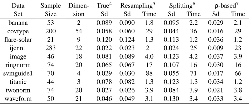
To evaluate the variance estimator obtained by the perturbation-resampling procedure, we esti-mate the standard deviation of 5-fold cross-validation error based only on the first partition of each data set. We also obtain the 5-fold cross-validation estimates of the SVM classifier on the rest 99 partitions, and the results are used to calculate the sample standard deviation of the cross-validation estimator, which is regarded as the true value. For comparison, we estimate the standard deviation based on two other methods proposed by Nadeau and Bengio (2003) using the first partition of each data set. The first approach is performed by randomly splitting data into two distinct sets (we name it ”splitting” method here), and the second approach is based on the approximation of a so-called
statisticρ(we name it ”ρ-based” method here). The description of the data sets, the standard
de-viations estimated by different methods, and their computational efficiencies are shown in Table 3. Computational time is tested on a PC with a Pentium 4 running at 2.8GHz and 512MB of RAM.
The results in Table 3 suggest that the perturbation-resampling based estimate of the standard deviation using only the first partition of each data set is rather close to the sample standard de-viation estimated using the entire data set. To the contrary, the standard dede-viation estimated by
splitting the data set tends to be biased upward, while theρ-based method tends to underestimate
the standard deviation of the cross-validation error. In the results shown above, 1,000 times of
ran-domly splitting or resampling are used in all the three methods, and as a result, the actual computa-tional efficiencies of different methods are comparable. This study demonstrates that the proposed perturbation-resampling procedure can be an accurate and efficient way to estimate the variance of the cross-validation error.
4.3 Example in Kernel Selection
To illustrate the application of the proposed procedure in model comparison, we perform kernel selection for SVM classifiers on simulated data. Samples{(X1i,X2i); i=1, ...,n}are generated from a uniform distribution on two-dimensional area[0,1]×[0,1]. For data type 1, two classes of samples
are separated by the curve corresponding to a linear function, X1+X2=1, with a few exceptions
introduced as ”noise”. For data type 2, the separating curve corresponds to a cubic function X13+
Data Sample Dimen- True4 Resampling5 Splitting6 ρ-based7
Set Size sion Sd Sd Time Sd Time Sd Time
banana 53 2 0.089 0.090 1.8 0.095 2.2 0.029 2.1
covtype 200 54 0.058 0.060 29 0.044 36 0.016 29
flare-solar 21 9 0.120 0.124 1.3 0.113 1.2 0.036 1.2
ijcnn1 283 22 0.022 0.023 21 0.024 25 0.009 23
image 46 18 0.081 0.089 4.0 0.123 4.2 0.037 3.9
ringnorm 74 20 0.065 0.067 17 0.107 16 0.030 16
svmguide1 70 4 0.029 0.030 88 0.055 71 0.017 66
titanic 44 3 0.078 0.082 1.3 0.123 1.3 0.034 1.2
twonorm 74 20 0.027 0.026 3.9 0.084 3.9 0.021 3.8
waveform 50 21 0.046 0.049 3.1 0.130 3.4 0.033 3.4
Table 3: Estimating the standard deviation of the 5-fold cross-validation error using different meth-ods (computational time is shown in seconds).
kernel, while the cubic polynomial kernel might perform better when classifying samples from data type 2. We generate each type of data with sample size n equal to 100 and 200, respectively.
Polynomial kernels can be generalized as K(Xi,Xj) = (γX0iXj+b)d, where Xi and Xj, i,j=
1, . . . ,n, are input vectors. In our study, we choose the hyper-parameters asγ=1/n, b=0, and
d=3. Then we apply the SVM algorithm by using the linear kernel and the polynomial kernel
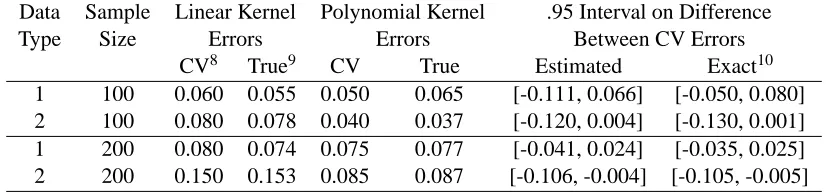
with optimal hyper-parameter C chosen by a cross-validation procedure, respectively. To make inference about the performances of different kernels, we use the model comparison procedure introduced in Section 3.3 to obtain 95% confidence intervals for the difference in cross-validation errors when using different kernels. We also compute the true prediction errors, together with the exact confidence intervals on the difference between their cross-validated estimates, based on the prediction results of 1,000 replications of simulated data sets for each setting. In Table 4, we report the 10-fold cross-validation errors by using linear and polynomial kernels, the 95% confidence intervals on the difference between errors, and their respective true values.
For the first type of data, although the polynomial kernel could potentially lead to slightly lower error rates compared to the linear kernel, 95% confidence intervals for error difference are quite tight around zero. This suggests that the classifiers obtained based on these two types of kernels have similar accuracies as we expect. On the other hand, for the second type of data, 95% confidence intervals for error differences tend to deviate downward from zero, which indicates that the
polyno-mial kernel indeed performs better than the linear kernel. (At the significant level of 0.05, n=100
is not sufficient to conclude this, whereas n=200 allows to make the above statement.) These
4. The true standard deviation (Sd) is calculated based on 5-fold cross-validation errors estimated on the rest 99 parti-tions of the data.
5. Standard deviation (Sd) and computation time (Time) are obtained by applying perturbation-resampling method on the first partition of the data.
6. Standard deviation (Sd) and computation time (Time) are obtained by applying splitting method (Nadeau and Bengio, 2003) on the first partition of the data.
Data Sample Linear Kernel Polynomial Kernel .95 Interval on Difference
Type Size Errors Errors Between CV Errors
CV8 True9 CV True Estimated Exact10
1 100 0.060 0.055 0.050 0.065 [-0.111, 0.066] [-0.050, 0.080]
2 100 0.080 0.078 0.040 0.037 [-0.120, 0.004] [-0.130, 0.001]
1 200 0.080 0.074 0.075 0.077 [-0.041, 0.024] [-0.035, 0.025]
2 200 0.150 0.153 0.085 0.087 [-0.106, -0.004] [-0.105, -0.005]
Table 4: Kernel selection based on the interval estimates of the difference in cross-validation errors.
conclusions are consistent with the intuitions behind the data generating procedure. In particular, the predicted results are consistent with the true values of both point and interval estimates obtained by simulating a large number of data sets. This study serves as an example to demonstrate how to use the proposed model comparison procedure to choose an appropriate kernel in constructing SVM classifiers.
4.4 Example in the Genotypic Testing for Drug Resistance
In this section, we give an example to show how the proposed procedure can be used in selecting important markers in the genotypic testing for HIV protease inhibitor (PI) resistance on the HIV RT and Protease Sequence Database (Rhee et al., 2003). First, we divide the sample set into two classes by labeling each protease sequence sample with 99 amino acids as either ”resistant” or ”susceptible”, depending on whether the resistance factor of the sample exceeds a certain drug-specific cutoff value or not (Beerenwinkel et al., 2002). Then, we predict the resistance to seven FDA-approved PIs using 10 sites on the substrate binding cleft or its flap that are reported to cause resistance by reducing the binding affinity between the inhibitor and the mutant protease enzyme.
Aside from these mutations, mutation information at site 90, denoted by X(90), on the protease
sequence has been reported to either contribute to or directly confer in vitro and in vivo resistance to each of the seven approved PIs, but the mechanism by which these mutations cause PI resistance is still not known. It is interesting to assess the incremental value of X(90)in predicting HIV drug
resistance. To this end, we compare the prediction errors for the models with and without X(90)and
evaluate the incremental value of X(90) based on the reduction in the prediction error, denoted by
∆X(90). We obtain the point and interval estimates of∆X(90) based on the model comparison method discussed in Section 3.3 with 10-fold cross-validation. In both cases, the hyper-parameter C is chosen by using a cross-validation procedure, respectively.
The results in Table 5 show that the 95% confidence intervals for∆X(90) are tight around zero for drugs APV, ATV, and LPV, which indicates that X(90)adds rather modest value, if any, on top of other variables, for predicting resistance to these drugs. On the other hand, by including information on X(90), the prediction of drug resistance to IDV and RTV can be significantly improved in a sense that
8. 10-fold cross-validation errors are computed.
9. The true errors are estimated based on the prediction results of 1,000 replications of simulated data sets for each setting.
Drug Sample Resistant Without Site 90 With Site 90 .95 Interval
Name Size Fraction Error .95 Interval Error .95 Interval for Difference
APV 577 38.1% 0.149 [0.130,0.202] 0.147 [0.129,0.198] [-0.025,0.025]
ATV 142 51.4% 0.261 [0.195,0.403] 0.197 [0.135,0.270] [-0.110,0.022]
IDV 579 50.6% 0.123 [0.108,0.163] 0.081 [0.067,0.133] [-0.063,-0.006]
LPV 253 74.7% 0.119 [0.090,0.236] 0.115 [0.078,0.167] [-0.032,0.027]
NFV 617 64.0% 0.113 [0.093,0.147] 0.092 [0.076,0.130] [-0.050,0.001]
RTV 510 50.2% 0.098 [0.069,0.123] 0.057 [0.039,0.090] [-0.060,0.000]
SQV 598 43.6% 0.172 [0.146,0.211] 0.132 [0.113,0.166] [-0.080,0.002]
Table 5: Interval estimates for the prediction errors and their difference in the genotypic testing for HIV drug resistance with or without mutation information at site 90 on the protease sequence.
the 95% confidence intervals for∆X(90) tend to locate on the negative side of the zero point. These results are consistent with studies in literature (see Para et al., 2000; Shulman et al., 2002; Campo et al., 2003; Saah et al., 2003). Therefore, X(90)is an important marker for choosing antiretroviral drugs and therapies, and the roles played by X(90)in reducing the susceptibility of these two drugs
need to be further studied.
5. Discussion
In this paper, we propose procedures for making inference about the prediction error of SVM clas-sifiers based on cross-validated point estimators and their corresponding interval estimators. We es-tablish large sample theory for the cross-validated estimators, and present a perturbation-resampling procedure to construct the confidence interval for prediction errors. The proposed interval estimates
are obtained by approximating the spread of
W
with that of W . Alternatively, one may considerdirectly perturbing
W
to yield potentially better approximations. However, such a perturbationprocedure may be computationally intensive since a K-fold cross-validation scheme has to be con-ducted for each realization of the resampling weights. Results from extensive simulation studies suggest that the proposed point and interval estimators perform well in finite samples. Furthermore, through numerical studies, we demonstrate that the interval estimates provide much more informa-tion about the true underlying predicinforma-tion accuracy than the point estimates. Although it is unclear whether similar theoretical results hold for SVM classifier with the RBF kernel (see the discussion in Appendix B), the framework in this article is likely to be applicable to other inductive learning algorithms with different types of loss functions.
Acknowledgments
We thank the Editor and the reviewers for many helpful comments and invaluable suggestions. This work is supported in part by NSFC grants 60575014, 30625012, 60721003, the National Basic
Re-search Program (2004CB518605) and Hi-tech Research and Development Program
(2006AA02Z325) of China, and NIH grant R01 EB006195 of USA.
Appendix A. Consistency of ˆθand ˆD
In the following theorem, we will show that as n→∞, ˆθ→θ0and the training error ˆD(θˆ)will
con-verge to the absolute prediction error D0in probability. Without loss of generality, we assume that
g0(X) =P(Y =1|X)and the distribution function of X are continuously differentiable hereafter.
Theorem 1 Letθ0= (w00,b0)0=argminθ∈ΘQ(θ),Ωbe the input vector space, and Λ(Y,θ1) ={X∈Ω|[1−Y(w00X+b0)][1−Y(w01X+b1)]<0} forθ1= (w01,b1)0. Furthermore, we assume the following regularity condition:
P(Y =1,X∈Λ(1,θ1)) +P(Y =−1,X∈Λ(−1,θ1))>0 (12) for anyθ16=θ0. Then, as n→∞, ˆθ→θ0and ˆD(θˆ)→D0in probability.
Proof. In view of Theorem 2.1 of Newey and McFadden (1994, Section 2), we can establish the
convergence of ˆθ→θ0by showing that (a) Q(θ)has a unique minimizerθ0; and (b) ˆQn(θ)converges
to Q(θ)in probability, uniformly inθ.
For (a), we note that since Q(θ)is continuous with respect toθandΘis compact, it must have
a minimum withinΘ. Furthermore, it is easy to verify that for any a,b∈R,
(a+b)+≤a++b+, (13)
and a strict inequality holds if and only if ab<0. As a result, under condition (12), Q(θ)is a strictly
convex function atθ0, and thus has a unique minimizerθ0.
For (b), since ˆQn(θ) is also a convex function of θbecause of (13), and ˆQn(θ) converges in
probability to Q(θ) for each θ∈Θ, we have supθ∈Θ|Qˆn(θ)−Q(θ)|goes to zero in probability, a uniform convergence property for convex functions proved by Pollard (1991, Section 6). This concludes the proof for the convergence of ˆθtoθ0in probability.
It remains to show the consistency of ˆD(θˆ)for D0. Since g0(X)is continuously differentiable, E|Y0−Yˆ(X0,θ)| is continuously differentiable in θ with bounded derivatives. Moreover, since 0≤E|Y0−Yˆ(X0,θ)| ≤2, it follows from a uniform law of large numbers (Pollard, 1990, Chap-ter 8) that supθ∈Θ|Dˆ(θ)−E|Y0−Yˆ(X0,θ)|| →0 in probability. This, coupled with the convergence of ˆθtoθ0, implies that ˆD(θˆ)−D0→0 in probability.
The regularity condition in (12) guarantees the existence and uniqueness of the minimizer to
the objective function. This condition states that any deviation of the parameterθfrom the
mini-mizerθ0will always result in the change of output labels of certain samples. Given the continuous
Appendix B. Large Sample Distribution for ˆD
With the assumption that g0(X) =P(Y =1|X)and the distribution function of X are continuously differentiable, we have∇θ=θ0Q(θ) =−E{Y I(Y f(X;θ0)<1)(X0,1)0}, which is also differentiable,
almost everywhereθ∈Θ. Thus, Q(θ)is twice differentiable almost everywhereθ∈Θ. Let H be the
Hessian matrix of Q(θ)atθ0, d(θ) =E{Dˆ(θ)}and ˙d(θ) =∇d(θ), we prove the following theorem:
Theorem 2 Under the regularity condition (12) in Theorem 1, the distribution of W is asymptotically
equivalent to n−1/2∑ni=1ηiand converges to a zero mean normal with variance E(η2i), where
ηi=|Yi−Yˆ(Xi,θ0)| −D0−d˙(θ0)H−1Mi(θ0), (14) and Mi(θ0) =−YiI(Yif(Xi;θ0)<1)(X0i,1)0+2λn(w00,0)0.
Proof. Under the regularity condition, the limiting objective function Q(θ)is strictly convex atθ0, and thus its Hessian matrix H atθ0is positive definite. To derive the asymptotic distribution theory for W , we first show that
√
n(θˆ−θ0) =−n−1/2H−1
n
∑
i=1
Mi(θ0) +op(1), (15)
where Mi(θ0) =−YiI(Yif(Xi;θ0)<1)(X0i,1)0+2λn(w00,0)0. To this end, let Z= (X0,Y)0, t= (w0t,bt)0, and write
[1−Y f(X;θ0+t)]+−[1−Y f(X;θ0)]+=B(Z)0t+R(Z,t), (16)
where B(Z) =−Y I(Y f(X;θ0)<1)(X0,1)0, and
R(Z,t) = {1−Y f(X;θ0+t)}[I{Y f(X;θ0+t)<1} −I{Y f(X;θ0)<1}].
Noting that R(Z,0) =0, and that the distribution function of X and the conditional probability mass function of Y given X are continuous differentiable, it is easy to verify that
ER(Z,t) =1 2t
0Ht+o(ktk2)and ER(Z,t)2=O(ktk3).
Furthermore, EB(Z) is just the first order derivative of Q(θ) at θ0, thus EB(Z) =0. Let Zi =
(X0i,Yi)0, s= (w0s,bs)0, and An(s) =∑ni=1{[1−Yif(Xi;θ0+s/√n)]++λn(w0+ws/√n)0(w0+ws/√n)
−[1−Yif(Xi;θ0)]+−λnw00w0}. An(s) is convex with respect to s because of (13), and it is
mini-mized by√n(θˆn−θ0). Note first that nER(Z,s/√n) =12s0Hs+rn,0(s), where rn,0(s) =o(ksk2)→0 for fixed s. Accordingly, using (16),
An(s) = n
∑
i=1
{[B(Zi) +2λn(w00,0)0]0s/ √
n+R(Zi,s/√n)−ER(Zi,s/√n)}
+nER(Z,s/√n) +λnw0sws
= Un0s+1 2s
0Hs+r
n,0(s) +rn,1(s) +rn,2(s),
where Un=n−1/2∑ni=1{B(Zi) +2λn(w00,0)0}=n−1/2∑ni=1Mi(θ0), rn,2(s) =λnw0sws, and rn,1(s) =
∑n
mean is zero and its variance is∑ni=1var{R(Zi,s/√n)}=o(ksk2). Moreover, rn,2(s) also tends to
be zero in probability whenλn→0. Since An(s)is a convex function, H is positive definite, and the
covariance matrix var(X)is finite, it follows from the Basic Corollary of Hjort and Pollard (1993)
that (15) holds.
Secondly, we show that the class of functions indexed byθ,ℑ={|Y−Yˆ(X,θ)|:kθ−θ0k ≤δ} is a Donsker class, where δ is a given positive number and ˆY(X,θ) =sign(w0X+b). Both of the classes of function {1+Yˆ(X,θ):kθ−θ0k ≤δ} and {1−Yˆ(X,θ):kθ−θ0k ≤δ} are VC classes (van der Vaart and Wellner, 1996, Lemma 2.6.15), and hence are Donsker. Note that in this caseℑ={I(Y =−1)[1+Yˆ(X,θ)] +I(Y =1)[1−Yˆ(X,θ)]:kθ−θ0k ≤δ}, and therefore is a Donsker class. It follows that n1/2[Dˆ(θ)−d(θ)], a process inθ, converges weakly to a zero mean
Gaussian process and thus is stochastic equicontinuous atθ0. This, coupled with (15), implies that
n1/2{Dˆ(θˆ)−D0}=n1/2[Dˆ(θˆ)−Dˆ(θ0)] +n1/2[Dˆ(θ0)−D0]is asymptotically equivalent to n1/2{Dˆ(θ0)−D0}+d˙(θ0)n1/2(θˆ−θ0)'n−1/2
n
∑
i=1
ηi,
where
ηi=|Yi−Yˆ(Xi,θ0)| −D0−d˙(θ0)H−1Mi(θ0).
Here and in the sequel, we use the notation a 'b to denote that a =b+op(1). Thus, W =
n1/2{Dˆ(θˆ)−D0}converges in distribution to a zero mean normal random variable. Since the limiting variance of W isσ2=E(η2
i)and n−1∑ni=1η2i converges toσ2in probability
(based on the law of large numbers), one may estimateσ2 by n−1∑ni=1η2i. Furthermore, it is not difficult to show that n−1∑ni=1(η2
i −ηˆ2i)→0 since we expect that all the empirical estimates of the
theoretical quantities inηiare consistent. We note that although n−1∑ni=1ηˆ2i is a consistent estimator
ofσ2, we approximateσ2based on the resampling method, not n−1∑ni=1ηˆ2
i.
For a more general case, when the prediction function f(X)in (1) is not a linear function of the input vector X, one can rewrite the prediction function in the form of f(X) =w0Φ(X) +b, whereΦ is a mapping from the input vector space to a ”feature space”
H
. Given that the expectation EΦ(X), the covariance matrix var(Φ(X)), and the VC dimension of f(X)are all finite (for example, whenΦ is a mapping corresponding to a polynomial kernel function), and coupled with the fact that a
{0,1}-valued class of functions is a uniform Donsker class if and only if its VC dimension is finite (Dudley, 1999), one can prove all the results given above using similar arguments. Note that when it comes to construct SVM classifier using the RBF kernel, however, these conditions cannot be satisfied because of the infinite-dimensional feature space of the RBF kernel.
Appendix C. Large Sample Property of ˆ
D
In this appendix, we will show that the distribution of
W
is asymptotically equivalent to that of Wbased on training error.
Theorem 3
W
in (8) is asymptotically equivalent to W in (6).variables uniformly distributed over{1, . . . ,K}, independent of the data, which satisfy∑ni=1I(ξi=
k)'n/K,k=1, . . . ,K. Conditionally on{ξi; i=1, . . . ,n}, it follows from similar arguments in
Appendix B that
ˆ
θ(−k)−θ0=− K n(K−1)H−
1
∑
ni=1
I(ξi6=k)Mi(θ0) +op(n−1/2).
Then using the same argument as given for n1/2{Dˆ(θˆ)−D
0}, one can show that n1/2{Dˆ(k)(θˆ(−k))−
D0}is asymptotically equivalent to
n1/2{Dˆ(k)(θ0)−D0}+d˙(θ0)n1/2(θˆ(−k)−θ0)'n1/2
n
∑
i=1
ηki,
where
ηki=I(ξi=k)K{|Yi−Yˆ(Xi,θ0)| −D0}+I(ξi6=k)
K
K−1d˙(θ0)H
−1M
i(θ0).
It follows that n1/2(
D
ˆ −D0)'n−1/2∑ni=1(∑Kk=1K−1ηki). Since∑Kk=1I(ξi=k) =1 and∑Kk=1I(ξi6=k) =K−1, it is straightforward to show that
n−1/2
n
∑
i=1 (
K
∑
k=1
K−1ηki) = n−1/2 n
∑
i=1
|Yi−Yˆ(Xi,θ0)| −D0+d˙(θ0)H−1Mi(θ0)
= n−1/2
n
∑
i=1
ηi.
Appendix D. Justification for the Perturbation-Resampling Procedure
Here, we give a brief justification for the perturbation-resampling approach presented in Section 3.2. For formal justification of the approach, please see similar but more rigorous derivations given in Park and Wei (2003) and Cai et al. (2005).
To justify the resampling method, we first note that it follows from the arguments in Appendix B that
√
n(θˆ−θ0) =−n−1/2H−1
n
∑
i=1
Mi(θ0) +op(1),
and that
√
n(θ∗−θ0) =−n−1/2H−1
n
∑
i=1
GiMi(θ0) +op(1),
where Mi(θ0) =−YiI(Yif(Xi;θ0)<1)(X0i,1)0+2λn(w00,0)0.
Then, consider the unconditional version of W∗. Let D∗(θ) =n−1∑ni=1{|Yi−Yˆ(Xi,θ)|Gi},
ˆ
from the same population of(X,Y), and the expectation E is with respect to{(Xi,Yi); i=1, . . . ,n}
and(X0,Y0). As ˆθconverges toθ0and ˆD(θˆ)converges to D0, it is straight forward to show that W∗ = n1/2(D∗(θ∗)−D∗(θ0))−n1/2(Dˆ(θˆ)−Dˆ(θ0))
+n1/2(D∗(θ0)−Dˆ(θ0))−n−1/2
n
∑
i=1 ˆ
D(θˆ)(Gi−1)
' d˙(θ0)n1/2(θ∗−θ0)−d˙(θ0)n1/2(θˆ−θ0) +n−1/2
n
∑
i=1
|Yi−Yˆ(Xi,θ0)|(Gi−1)−n−1/2 n
∑
i=1
D0(Gi−1)
' n−1/2
n
∑
i=1
{|Yi−Yˆ(Xi,θ0)| −D0}(Gi−1)−d˙(θ0)n−1/2H−1
n
∑
i=1
Mi(θ0)(Gi−1)
= n−1/2
n
∑
i=1
ηi(Gi−1),
whereηi=|Yi−Yˆ(Xi,θ0)| −D0−d˙(θ0)H−1Mi(θ0).
Conditionally on the data, it follows from the Multiplier Central Limit Theorem (van der Vaart
and Wellner, 1996, Chapter 2.9) that the conditional distribution of W∗converges to a normal with
mean 0 and variance n−1∑ni=1η2i, which are the same as the unconditional distribution of W (or its cross-validation counterpart
W
). This implies that forε>0, there exists an N0 such that when n>N0, the probability, with respect to samplesS
={(Xi,Yi); i=1, . . . ,n}, of the eventsup
u∈R|
P(W∗≤u|
S
)−P(W ≤u)|<ε,is at least 1−ε.
References
L. Beerenwinkel, B. Schmidt, H. Walter, R. Kaiser, T. Lengauer, D. Hoffmann, K. Korn, and J. Sel-big. Diversity and complexity of HIV-1 drug resistance: A bioinformatics approach to predicting phenotype from genotype. Proceedings of the National Academy of Sciences U.S.A., 99:8271– 8276, 2002.
Y. Bengio and Y. Grandvalet. No unbiased estimator of the variance of k-fold cross-validation. Journal of Machine Learning Research, 5:1089–1105, 2004.
O. Bousquet and A. Elisseeff. Stability and generalization. Journal of Machine Learning Research, 2:499–526, 2002.
T. Cai, L. Tian, and L. J. Wei. Semiparametric Box-Cox power transformation models for censored survival observations. Biometrika, 92:619–632, 2005.
C. C. Chang and C. H. Lin. Libsvm—a library for support vector machine. Available at http://www.csie.ntu.edu.tw/cjlin/libsvm/, 2001.
T. Dietterich. Approximate statistical tests for comparing supervised classification learning algo-rithms. Neural Computation, 10:1895–1923, 1998.
R. M. Dudley. Uniform Central Limit Theorems. Cambridge, U.K.: Cambridge University Press, 1999.
B. Efron. Bootstrap methods: Another look at the jackknife. The Annals of Statistics, 7:1–26, 1979.
B. Efron. How biased is the apparent error rate of a prediction rule. Journal of the American Statistical Association, 81:461–470, 1986.
B. Efron. Better bootstrap confidence intervals. Journal of the American Statistical Association, 82: 171–185, 1987.
B. Efron and R. Tibshirani. Cross-validation and the bootstrap: Estimating the error rate of a prediction rule. Technical report, Stanford University, 1995.
B. Efron and R. Tibshirani. Improvements on cross-validation: The .632+ bootstrap method. Jour-nal of the American Statistical Association, 92:548–560, 1997.
W. J. Fu, R. J. Carroll, and S. Wang. Estimating misclassification error with small samples via bootstrap cross-validation. Bioinformatics, 21:1979–1986, 2005.
P. Hall and Y. Maesono. A weighted bootstrap approach to bootstrap iteration. Journal of the Royal Statistical Society Series B, 62:137–144, 2000.
P. Hall and E. Mammen. On general resampling algorithms and their performance in distribution estimation. The Annals of Statistics, 22:2011–2030, 1994.
N. L. Hjort and D. Pollard. Asymptotics for minimizers of convex processes. Technical report, Yale University, 1993.
M. Kearns and D. Ron. Algorithmic stability and sanity check bounds for leave-one-out cross-validation. Neural Computation, 11:1427–1453, 1999.
R. Y. Liu. Bootstrap procedures under some non-i.i.d. models. The Annals of Statistics, 16:1696– 1708, 1988.
S. Mika, G. R ¨atsch, J. Weston, B. Sch ¨olkopf, and K. R. M ¨uller. Fisher discriminant analysis with kernels. In Neural Networks for Signal Processing IX, pages 41–48, 1999.
A. Molinaro, R. Simon, and R. Pfeiffer. Prediction error estimation: A comparison of resampling methods. Bioinformatics, 21:3301–3307, 2005.
W. Newey and D. McFadden. Large sample estimation and hypothesis testing. In D. McFadden and R. Engler, editors, Handbook of Econometrics IV, pages 2113–2245. Amsterdam: North Holland, 1994.
M. F. Para, D. V. Glidden, R. Coombs, A. Collier, J. Condra, C. Craig, R. Bassett, R. Leavitt, S. Snyder, V. J. McAuliffe, and C. Boucher. Baseline human immunodeficiency virus type I phenotype, genotype, and RNA response after switching from long-term hard-capsule saquinavir to indinavir or soft-gel-capsule saquinavir in AIDS clinical trials group protocol 333. Journal of Infectious Diseases, 182:733–743, 2000.
Y. Park and L. J. Wei. Estimating subject-specific survival functions under the accelerated failure time model. Biometrika, 90:717–723, 2003.
D. Pollard. Empirical Process: Theory and Applications. Hayward, CA: Institute of Mathematical Statistics, 1990.
D. Pollard. Asymptotics for least absolute deviation regression estimators. Econometric Theory, 7: 186–199, 1991.
J. Reunanen. Overfitting in making comparisons between variable selection methods. Journal of Machine Learning Research, 3:1371–1382, 2003.
S. Y. Rhee, M. J. Gonzales, R. Kantor, B. J. Betts, J. Ravela, and R. W. Shafer. Human immunode-ficiency virus reverse transcriptase and protease sequence database. Nucleic Acids Research, 31: 298–303, 2003.
D. Rubin. The bayesian bootstrap. The Annals of Statistics, 9:130–134, 1981.
A. J. Saah, D. W. Haas, M. J. DiNubile, J. Chen, D. J. Holder, R. R. Rhodes, M. Shivaprakash, K. K. Bakshi, R. M. Danovich, D. J. Graham, and J. H. Condra. Treatment with indinavir, efavirenz, and adefovir after failure of nelfinavir therapy. Journal of Infectious Diseases, 187:1157–1162, 2003.
J. Shao. Bootstrap model selection. Journal of the American Statistical Association, 91:655–665, 1996.
N. Shulman, A. Zolopa, D. Havlir, A. Hsu, C. Renz, S. Boller, P. Jiang, R. Rode, J. Gallant, E. Race, D. J. Kempf, and E. Sun. Virtual inhibitory quotient predicts response to ritonavir boost-ing of indinavir-based therapy in human immunodeficiency virus-infected patients with ongoboost-ing viremia. Antimicrobial Agents and Chemotherapy, 146:3907–3916, 2002.
I. Steinwart. Support vector machines are universally consistent. Journal of Complexity, 18:768– 779, 2002.
A. W. van der Vaart and J. A. Wellner. Weak Convergence and Empirical Processes. New York: Springer-Verlag Inc., 1996.
V. N. Vapnik. The Nature of Statistical Learning Theory. New York: Springer, 1995.
S. Varma and R. Simon. Bias in error estimation when using cross-validation for model selection. BMC Bioinformatics, 7:91, 2006.