Online Learning with Sample Path Constraints
Shie Mannor∗ [email protected]
Department of Electrical and Computer Engineering McGill University
Qu´ebec H3A-2A7
John N. Tsitsiklis [email protected]
Laboratory for Information and Decision Systems Massachusetts Institute of Technology
Cambridge, MA 02139
Jia Yuan Yu [email protected]
Department of Electrical and Computer Engineering McGill University
Qu´ebec H3A-2A7
Editor: G´abor Lugosi
Abstract
We study online learning where a decision maker interacts with Nature with the objective of max-imizing her long-term average reward subject to some sample path average constraints. We define the reward-in-hindsight as the highest reward the decision maker could have achieved, while sat-isfying the constraints, had she known Nature’s choices in advance. We show that in general the reward-in-hindsight is not attainable. The convex hull of the reward-in-hindsight function is, how-ever, attainable. For the important case of a single constraint, the convex hull turns out to be the highest attainable function. Using a calibrated forecasting rule, we provide an explicit strategy that attains this convex hull. We also measure the performance of heuristic methods based on non-calibrated forecasters in experiments involving a CPU power management problem.
Keywords: online learning, calibration, regret minimization, approachability
1. Introduction
We consider a repeated game from the viewpoint of a decision maker (player P1) who plays against Nature (player P2). The opponent (Nature) is “arbitrary” in the sense that player P1 has no pre-diction, statistical or strategic, of the opponent’s choice of actions. This setting was considered by Hannan (1957), in the context of repeated matrix games. Hannan introduced the Bayes utility with respect to the current empirical distribution of the opponent’s actions, as a performance goal for adaptive play. This quantity, defined as the highest average reward that player P1 could have achieved, in hindsight, by playing some fixed action against the observed action sequence of player P2. Player P1’s regret is defined as the difference between the highest average reward-in-hindsight that player P1 could have hypothetically achieved, and the actual average reward obtained by player P1. It was established in Hannan (1957) that there exist strategies whose regret converges to zero as
the number of stages increases, even in the absence of any prior knowledge on the strategy of player P2. For recent advances on online learning, see Cesa-Bianchi and Lugosi (2006).
In this paper we consider regret minimization under sample-path constraints. That is, in addition to maximizing the average reward, or more precisely, minimizing the regret, the decision maker has some side constraints that need to be satisfied on the average. In particular, for every joint action of the players, there is an additional penalty vector that is accumulated by the decision maker. The decision maker has a predefined set in the space of penalty vectors, which represents the accept-able tradeoffs between the different components of the penalty vector. An important special case arises when the decision maker wishes to keep some constrained resource below a certain threshold. Consider, for example, a wireless communication system where the decision maker can adjust the transmission power to improve the probability that a message is received successfully. Of course, the decision maker does not know a priori how much power will be needed (this depends on the behavior of other users, the channel conditions, etc.). Still, a decision maker is usually interested in both the rate of successful transmissions, and in the average power consumption. In an often consid-ered variation of this problem, the decision maker wishes to maximize the transmission rate, while keeping the average power consumption below some predefined threshold. We refer the reader to Mannor and Shimkin (2004) and references therein for a discussion of constrained average cost stochastic games and to Altman (1999) for constrained Markov decision problems. We note that the reward and the penalty are not treated the same; otherwise they could have been combined into a single scalar value, resulting in a much simpler problem.
The paper is organized as follows. In Section 2, we present formally the basic model, and provide a result that relates attainability with the value of the game. In Section 3, we provide an example where the reward-in-hindsight cannot be attained. In light of this negative result, in Section 4 we define the closed convex hull of the reward-in-hindsight, and show that it is attainable. Furthermore, in Section 5, we show that when there is a single constraint, this is the maximal attainable objective. In Section 6, we provide a simple strategy, based on calibrated forecasting, that attains the closed convex hull. Section 7 presents heuristic algorithms derived from an online forecaster, while incorporating strictly enforced constraints. The application of the algorithms of Section 7 to a power management domain is presented in Section 8. We finally conclude in Section 9 with some open questions and directions for future research.
2. Problem Definition
We consider a repeated game against Nature, in which a decision maker tries to maximize her reward, while satisfying some constraints on certain time-averages. The underlying stage game is a game with two players: P1 (the decision maker of interest) and P2 (who represents Nature and is assumed arbitrary). For our purposes, we only need to define rewards and constraints for P1.
A constrained game with respect to a set T is defined by a tuple(A,B,R,C,T)where:
1. A is the set of actions of P1; we will assume A={1,2, . . . ,|A|}.
2. B is the set of actions of P2; we will assume B={1,2, . . . ,|B|}.
3. R is an |A| × |B| matrix where the entry R(a,b) denotes the expected reward obtained by
P1, when P1 plays action a∈A and P2 action b∈B. The actual rewards obtained at each
distributed according to a probability law PrR(· |a,b). Furthermore, the reward streams for different pairs(a,b)are statistically independent.
4. C is an|A| × |B|matrix, where the entry C(a,b)denotes the expected d-dimensional penalty
vector incurred by P1, when P1 plays action a∈A and P2 action b∈B. The actual penalty
vectors obtained at each play of actions a and b are assumed to be IID random variables, with
finite second moments, distributed according to a probability law PrC(· |a,b). Furthermore,
the penalty vector streams for different pairs(a,b)are statistically independent.
5. T is a set inRd within which we wish the average of the penalty vectors to lie. We assume
that T is convex and closed. Since the entries of C are bounded, we will also assume, without loss of generality, that T is bounded.
The game is played in stages. At each stage t, P1 and P2 simultaneously choose actions at∈A
and bt∈B, respectively. Player P1 obtains a reward rt, distributed according to PrR(· |at,bt), and a penalty ct, distributed according to PrC(· |at,bt). We define P1’s average reward by time t to be
ˆrt = 1
t
t
∑
τ=1
rτ, (1)
and P1’s average penalty vector by time t to be
ˆ
ct = 1
t
t
∑
τ=1
cτ. (2)
A strategy for P1 (resp. P2) is a mapping from the set of all possible past histories to the set of mixed actions on A (resp. B), which prescribes the (mixed) action of that player at each time t, as a
function of the history in the first t−1 stages. Loosely, P1’s goal is to maximize the average reward
while having the average penalty vector converge to T , pathwise:
lim sup t→∞ dist
(cˆt,T)→0, a.s., (3)
where dist(·) is the point-to-set Euclidean distance, that is, dist(x,T) =infy∈Tky−xk2, and the
probability measure is the one induced by the policy of P1, the policy of P2, and the randomness in the rewards and penalties.
We will often consider the important special case where T ={c∈Rd: c≤c0}, for some given
c0∈Rd, with the inequality interpreted component-wise. We simply call such a game a constrained
game with respect to (a vector) c0. For that special case, the requirement (3) is equivalent to:
lim sup t→∞
ˆ
ct≤c0, a.s..
For a set D, we will use the notation∆(D)to denote the set of all probability measures on D. If
D is finite, we will identify∆(D)with the set of probability vectors of the same size as D. If D is a
2.1 Reward-in-hindsight
We define ˆqt ∈∆(B)as the empirical distribution of P2’s actions by time t, that is,
ˆ
qt(b) = 1
t
t
∑
τ=1
1{bt=b}, b∈B. (4)
If P1 knew in advance that ˆqt will equal q, and if P1 were restricted to using a fixed action, then
P1 would pick an optimal response (generally a mixed action) to the mixed action q, subject to the
constraints specified by T . In particular, P1 would solve the convex program1
max
p∈∆(A)
∑
a,bp(a)q(b)R(a,b), (5)s.t.
∑
a,b
p(a)q(b)C(a,b)∈T.
By playing a p that solves this convex program, P1 would meet the constraints (up to small fluctua-tions that are a result of the randomness and the finiteness of t), and would obtain the maximal
aver-age reward. We are thus led to define P1’s reward-in-hindsight, which we denote by r∗:∆(B)7→R,
as the optimal objective value in the program (5), as a function of q. The function r∗is often referred
to as the Bayes envelope.
For the special case of a constrained game with respect to a vector c0, the convex constraint
∑a,bp(a)q(b)C(a,b)∈T is replaced by∑a,bp(a)q(b)C(a,b)≤c0(the inequality is to be interpreted component-wise).
The following examples show some of the properties of the Bayes envelope. Consider a 2×2
constrained game with respect to a scalar c0specified by:
(1,0) (0,1) (0,1) (1,0)
,
where each entry (pair) corresponds to (R(a,b),C(a,b)) for a pair of actions a and b. (Here a
and b correspond to a choice of row and column, respectively.) Suppose first that c0=1. In that
case the constraint does not play a part in the problem, and we are dealing with a version of the matching pennies game. So, if we identify q with the frequency of the first action, we have that
r∗(q) =max(q,1−q). Suppose now that c0=1/2. In this case, it is not difficult to show that r∗(q) =1/2, since P1 cannot take advantage of any deviation from q=1/2 while satisfying the constraint.
The next example involves a game where P2’s action does not affect the constraints; such games
are further discussed in Section 4.1. Consider a 2×2 constrained game with respect to a scalar c0,
specified by:
(1,1) (0,1) (0,0) (1,0)
,
where each entry (pair) corresponds to(R(a,b),C(a,b))for a pair of actions a and b. We identify
q with the frequency of the second action of P2 as before. Suppose first that c0=1. As before,
the constraint has no effect and r∗(q) =max(q,1−q). Suppose now that c0=1/2. It is not hard
to show that in this case r∗(q) =max(q,1/2). Finally, if c0=0, P1 is forced to choose the second
action; in this case, r∗(q) =q. The monotonicity of r∗(q)in c0is to be expected since the lower c0
is, the more stringent the constraint in Eq. (5).
2.2 The Objective
Formally, our goal is to attain a function r in the sense of the following definition. Naturally, the higher the function r, the better.
Definition 1 A function r :∆(B)7→Ris attainable by P1 in a constrained game with respect to a set T if there exists a strategyσof P1 such that for every strategyρof P2:
(i) lim inft→∞(ˆrt−r(qˆt))≥0, a.s.,and
(ii) lim supt→∞dist(cˆt,T)→0, a.s.,
where the almost sure convergence is with respect to the probability measure induced byσandρ.
In constrained games with respect to a vector c0we can replace (ii) in the definition with
lim sup t→∞ cˆt
≤c0, a.s.
2.3 The Value of the Game
In this section, we consider the attainability of a constant function r :∆(B)7→R, that is, r(q) =α,
for all q. We will establish that attainability is equivalent to havingα≤v, where v is a naturally
defined “value of the constrained game.”
We first introduce the assumption that P1 is always able to satisfy the constraint.
Assumption 1 For every mixed action q∈∆(B)of P2, there exists a mixed action p∈∆(A)of P1, such that:
∑
a,bp(a)q(b)C(a,b)∈T. (6)
For constrained games with respect to a vector c0, the condition (6) reduces to the inequality
∑a,bp(a)q(b)C(a,b)≤c0.
If Assumption 1 is not satisfied, then P2 can choose a q such that for every (mixed) action of P1, the constraint is violated in expectation. By repeatedly playing this q, P1’s average penalty vector will be outside T , and the objectives of P1 will be impossible to meet.
The following result deals with the attainability of the value, v, of an average reward repeated constrained game, defined by
v= inf
q∈∆(B)p∈∆(A):∑ sup
a,bp(a)q(b)C(a,b)∈T
∑
a,bp(a)q(b)R(a,b). (7)
Proposition 2 Suppose that Assumption 1 holds. Then,
(i) P1 has a strategy that guarantees that the constant function r(q)≡v is attained with respect
to T .
(ii) For every number v′>v there existsδ>0 such that P2 has a strategy that guarantees that
either lim inft→∞ˆrt <v′−δ or lim supt→∞dist(cˆt,T)>δ, almost surely. (In particular, the
constant function v′is not attainable.)
Proof The proof relies on Blackwell’s approachability theory (Blackwell, 1956a). We construct a
nested family of convex sets inRd+1 defined by Sα={(r,c)∈R×Rd: r≥α,c∈T}. Obviously,
Sα⊂Sβforα>β. Consider the vector-valued game inRd+1associated with the constrained game.
In this game, P1’s vector-valued payoff at time t is the d+1 dimensional vector mt= (rt,ct)and P1’s average vector-valued payoff is ˆmt= (ˆrt,cˆt). Since Sαis convex, it follows from approachability
the-ory for convex sets (Blackwell, 1956a) that each Sαis either approachable2or excludable.3 If Sαis
approachable, then Sβis approachable for everyβ<α. We define v0=sup{β|Sβis approachable}.
It follows that Sv0 is approachable (as the limit of approachable sets; see Spinat, 2002). By
Black-well’s theorem, for every q∈∆(B), an approachable convex set must intersect the set of feasible
payoff vectors when P2 plays q. Using this fact, it is easily shown that v0 equals v, as defined by
Eq. (7), and part (i) follows. Part (ii) follows because a convex set which is not approachable is excludable.
Note that part (ii) of the proposition implies that, essentially, v is the highest average reward P1 can attain while satisfying the constraints, if P2 plays an adversarial strategy. By comparing Eq. (7) with Eq. (5), we see that v=infqr∗(q). On the other hand, if P2 does not play adversarially, P1 may
be able to do better, perhaps attaining r∗(q). Our subsequent results address the question whether
this is indeed the case.
Remark 3 In general, the infimum and supremum in (7) cannot be interchanged. This is because the set of feasible p in the inner maximization depends on the value of q. Moreover, it can be shown that the set of (p,q) pairs that satisfy the constraint ∑a,bp(a)q(b)C(a,b)∈T is not necessarily
convex.
2. A set X is approachable if there exists a strategy for the agent such that for everyε>0, there exists an integer N such that, for every opponent strategy:
Pr dist 1
n n
∑
i=1 mt,X
!
≥εfor some n≥N
!
<ε.
3. A set X is excludable if there exists a strategy for the opponent such that there existsδ>0 such that for everyε>0, there exists an integer N such that, for every agent strategy:
Pr dist 1
n n
∑
i=1 mt,X
!
≥δfor all n≥N
!
2.4 Related Works
Notwithstanding the apparent similarity, the problem that we consider is not an instance of online convex optimization (Zinkevich, 2003; Hazan and Megiddo, 2007). In the latter setting, there is a
convex feasible domain
F
⊂Rn, and an arbitrary sequence of convex functions ft :F
→R. Atevery step t, the decision maker picks xt ∈
F
based on the past history, without knowledge of thefuture functions ft, and with the objective of minimizing the regret
T
∑
t=1ft(xt)−min y∈F
T
∑
t=1ft(y).
An analogy with our setting might be possible, by identifying xt and ft with at and bt, respectively,
and by somehow relating the feasibility constraints described by
F
to our constraints. However,this attempt seems to run into some fundamental obstacles. In particular, in our setting, feasibility is affected by the opponent’s actions, whereas in online convex optimization, the feasible domain
F
is fixed for all time steps. For this reason, we do not see a way to reduce the problem of onlinelearning with constraints to an online convex optimization problem, and given the results below, it is unlikely that such a reduction is possible.
3. Reward-in-Hindsight Is Not Attainable
As it turns out, the reward-in-hindsight cannot be attained in general. This is demonstrated by the
following simple 2×2 matrix game, with just a single constraint.
Consider a 2×2 constrained game specified by:
(1,−1) (1,1) (0,−1) (−1,−1)
,
where each entry (pair) corresponds to(R(a,b),C(a,b))for a pair of actions a and b. At a typical
stage, P1 chooses a row, and P2 chooses a column. We set c0=0. Let q denote the frequency
with which P2 chooses the second column. The reward of the first row dominates the reward of the second one, so if the constraint can be satisfied, P1 would prefer to choose the first row. This
can be done as long as 0≤q≤1/2, in which case r∗(q) =1. For 1/2≤q≤1, player P1 needs
to optimize the reward subject to the constraint. Given a specific q, P1 will try to choose a mixed
action that satisfies the constraint (on the average) while maximizing the reward. If we letαdenote
the frequency of choosing the first row, we see that the reward and penalty are:
r(α,q) =α−(1−α)q, c(α,q) =2αq−1,
respectively. We observe that for every q, r(α)and c(α)are monotonically increasing functions of
α. As a result, P1 will choose the maximalαthat satisfies c(α)≤0, which isα(q) =1/2q, and the
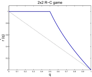
optimal reward is 1/2+1/2q−q. We conclude that the reward-in-hindsight is:
r∗(q) =
1, if 0≤q≤1/2,
1
2+
1
2q−q, if 1/2≤q≤1.
The graph of r∗(q)is the solid line in Figure 1.
0 0.1 0.2 0.3 0.4 0.5 0.6 0.7 0.8 0.9 1 0
0.2 0.4 0.6 0.8 1
q
r
*
(q
)
2x2 R−C game
Figure 1: The reward-in-hindsight of the constrained game. Here, r∗(q) is the solid line, and the
dotted line connects the two extreme values, for q=0 and q=1.
Proposition 4 If c0=0, then there exists a strategy for P2 such that r∗cannot be attained.
Proof Suppose that the opponent, P2, plays according to the following strategy. Initialize a counter
k=1. Let ˆαt be the empirical frequency with which P1 chooses the first row during the first t time
steps. Similarly, let ˆqt be the empirical frequency with which P2 chooses the second column during
the first t time steps.
1. While k=1 or ˆαt−1>3/4, P2 chooses the second column, and k is incremented by 1.
2. For the next k times, P2 chooses the first column. Then, reset the counter k to , and go back to Step 1.
We now show that if
lim sup t→∞
ˆ
ct ≤0, a.s.,
then a strict inequality holds for the regret:
lim inf t→∞ (ˆrt−r
∗(qˆ
t))<0, a.s.
0, we must have lim ˆαt≤1/2. But then, the condition ˆαt−1>3/4 will be eventually violated. This
shows that Step 2 is entered an infinite number of times. In particular, there exist infinite sequences
ti and ti′such that ti<ti′<ti+1 and (i) if ti<t≤ti′, P2 chooses the second column (Step 1); (ii) if
ti′<t≤ti+1, P2 chooses the first column (Step 2).
Note that Steps 1 and 2 last for an equal number of time steps. Thus, we have ˆqti =1/2, and
r∗(qˆti) =1, for all i. Furthermore, ti+1−t
′
i≤ti′, or ti′≥ti+1/2. Note that ˆαti′≤3/4, because otherwise
P2 would still be in Step 1 at time ti′+1. Thus, during the first ti+1time steps, P1 has played the
first row at most
3ti′/4+ (ti+1−ti′) =ti+1−ti′/4≤7ti+1/8
times. Due to the values of the reward matrix, we have lim supt→∞ˆrt <lim supi→∞ˆrti. In particular,
we have ˆrti+1 ≤7/8, and lim inft→∞(ˆrt−r ∗(qˆ
t))≤7/8−1<0.
Intuitively, the strategy that was described above allows P2 to force P1 to move, back and forth,
between the extreme points (q=0 and q=1) that are linked by the dotted line in Figure 1. Since
r∗(q) is not convex, and since the dotted line is strictly below r∗(q) for q=1/2, this strategy
precludes P1 from attaining r∗(q). We note that the choice of c0 is critical in this example. With
other choices of c0(for example, c0=−1), the reward-in-hindsight may be attainable.
4. Attainability of the Convex Hull
Since the reward-in-hindsight is not attainable in general, we have to settle for a more modest
objective. More specifically, we are interested in functions f :∆(B)→Rthat are attainable with
respect to a given constraint set T . As a target we suggest the closed convex hull of the reward-in-hindsight, r∗. After defining it, we prove that it is indeed attainable. In the next section, we will also show that it is the highest possible attainable function, when there is a single constraint.
Given a function f : X 7→R, over a convex domain X , its closed convex hull is the function
whose epigraph is
conv({(x,r): r≥ f(x)}),
where conv(D)is the convex hull, and D is the closure of a set D. We denote the closed convex hull
of r∗by rc.
We will make use of the following facts. Forming the convex hull and then the closure results in a larger epigraph, hence a smaller function. In particular, rc(q)≤r∗(q), for all q. Furthermore,
the closed convex hull is guaranteed to be continuous on∆(B). (This would not be true if we had
considered the convex hull, without forming its closure.) Finally, for every q in the interior of∆(B),
we have:
rc(q) = inf
q1,q2,...,qk∈∆(B),α1,...,αk
k
∑
i=1αir∗(qi) (8)
s.t. k
∑
i=1αiqi(b) =q(b), ∀b∈B,
αi≥0, i=1,2, . . . ,k, k
∑
i=1where k can be taken equal to|B|+2 by Caratheodory’s Theorem.
The following result is proved using Blackwell’s approachability theory. The technique is simi-lar to that used in other no-regret proofs (e.g., Blackwell, 1956b; Mannor and Shimkin, 2003), and is based on the convexity of a target set in an appropriately defined space.
Theorem 5 Let Assumption 1 hold for a given convex set T⊂Rd. Then rcis attainable with respect to T .
Proof Define the following game with vector-valued payoffs, where the payoffs belong to R×
Rd×∆(B)(a|B|+d+1 dimensional space, which we denote by
M
). Suppose that P1 plays at,P2 plays bt, P1 obtains an immediate reward of rt and an immediate penalty vector of ct. Then, the
vector-valued payoff obtained by P1 is
mt= (rt,ct,e(bt)),
where e(b) is a vector of zeroes, except for a 1 in its bth component. It follows that the average
vector-valued reward at time t, which we define as ˆmt =1t ∑tτ=1mτ, satisfies: ˆmt = (ˆrt,cˆt,qˆt), where ˆrt, ˆct, and ˆqt were defined in Eqs. (1), (2), and (4), respectively. Consider the sets:
B
1={(r,c,q)∈M
: r≥rc(q)},B
2={(r,c,q)∈M
: c∈T},and let
B
=B
1∩B
2. Note thatB
is a convex set. We claim thatB
is approachable. Let m :∆(A)×∆(B)→
M
describe the expected payoff in a single stage game, when P1 and P2 chooseactions p and q, respectively. That is,
m(p,q) =
∑
a,b
p(a)q(b)R(a,b),
∑
a,bp(a)q(b)C(a,b), q
.
Using the sufficient condition for approachability of convex sets (Blackwell, 1956a), it suffices to show that for every q there exists a p such that m(p,q)∈
B
. Fix q∈∆(B). By Assumption 1, thecon-straint∑a,bp(a)q(b)C(a,b)∈T is feasible, which implies that the program (5) has an optimal
solu-tion p∗. It follows that m(p∗,q)∈
B
. We now claim that a strategy that approachesB
also attains rc in the sense of Definition 1. Indeed, sinceB
⊆B
2we have that Pr(d(ct,T)>εinfinitely often) =0 for everyε>0. SinceB
⊆B
1and using the continuity of rc, we obtain lim inf(ˆrt−rc(qˆt))≥0.We note that Theorem 5 is not constructive. Indeed, a strategy that approaches
B
, based on anaive implementation Blackwell’s approachability theory, requires an efficient procedure for
com-puting the closest point in
B
,and therefore a computationally efficient description ofB
, which maynot be available (we do not know whether
B
can be described efficiently). This motivates thedevel-opment of the calibration based scheme in Section 6.
Remark 6 Convergence rate results also follow from general approachability theory, and are gen-erally of the order of t−1/3; see Mertens et al. (1994). It may be possible, perhaps, to improve upon this rate and obtain t−1/2, which is the best possible convergence rate for the unconstrained case. Remark 7 For every q∈∆(B), we have r∗(q)≥v, which implies that rc(q)≥v. Thus, attaining rc
4.1 Degenerate Cases
In this section, we consider the degenerate cases where the penalty vector is affected by only one of the players. We start with the case where P1 alone affects the penalty vector, and then discuss the case where P2 alone affects the penalty vector.
If P1 alone affects the penalty vector, that is, if C(a,b) =C(a,b′)for all a∈A and b,b′∈B, then r∗(q)is convex. Indeed, in this case, Eq. (5) becomes (writing C(a)for C(a,b))
r∗(q) = max
p∈∆(A):∑ap(a)C(a)∈T
∑
a,bp(a)q(b)R(a,b),
which is the maximum of a collection of linear functions of q (one function for each feasible p), and is therefore convex.
If P2 alone affects the penalty vector, that is, if c(a,b) =c(a′,b)for all b∈B and a,a′∈A, then
Assumption 1 implies that the constraint is always satisfied. Therefore,
r∗(q) = max
p∈∆(A)
∑
a,bp(a)q(b)R(a,b),which is again a maximum of linear functions, hence convex.
We conclude that in both degenerate cases, if Assumption 1 holds, then the reward-in-hindsight is attainable.
5. Tightness of the Convex Hull
We now show that rcis the maximal attainable function, for the case of a single constraint.
Theorem 8 Suppose that d=1, T is of the form T ={c|c≤c0}, where c0 is a given scalar, and that Assumption 1 is satisfied. Let ˜r :∆(B)7→Rbe a continuous attainable function with respect to the scalar c0. Then, rc(q)≥˜r(q)for all q∈∆(B).
Proof The proof is constructive, as it provides a concrete strategy for P2 that prevents P1 from
attaining ˜r, unless rc(q)≥˜r(q)for every q. Assume, in order to derive a contradiction, that there
exists some ˜r that violates the theorem. Since ˜r and rcare continuous, there exists some q0∈∆(B)
and someε>0 such that ˜r(q)>rc(q) +εfor all q in an open neighborhood of q0. In particular, q0 can be taken to lie in the interior of∆(B). Using Eq. (8), it follows that there exist q1, . . . ,qk∈∆(B)
andα1, . . . ,αk(with k≤ |B|+2, due to Caratheodory’s Theorem) such that
k
∑
i=1αir∗(qi)≤rc(q0) +ε
2 <˜r(q
0)−ε
2;
k
∑
i=1αiqi(b) =q0(b), ∀b∈B;
k
∑
i=1αi=1; αi≥0, ∀i.
Let τ be a large positive integer (τ is to be chosen large enough to ensure that the events of
interest occur with high probability, etc.). We will show that if P2 plays each qi for ⌈αiτ⌉ time
steps, in an appropriate order, then either P1 does not satisfy the constraint along the way or ˆrτ≤
−2 −1 0 1 2 0
0.5 1 1.5 2
Cost
Reward
pT C q = c
(a)
−2 −1 0 1 2
0 0.5 1 1.5 2
Cost
Reward p
T
C q = c
(b)
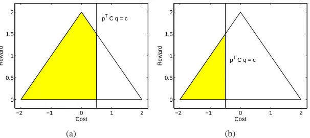
Figure 2: In either part (a) or (b) of the figure, we fix some q∈∆(B). The triangle is the set of
possible reward-cost pairs, as we vary p over the set∆(A). Then, for a given value c in
the upper bound on the cost (cf. 10), the shaded region is the set of reward-cost pairs that also satisfy the cost constraint.
We let qi, i=1, . . . ,k, be fixed, as above, and define a function fi:Rd→R∪ {−∞}as:
fi(c) = max
p∈∆(A)
∑
a,bp(a)qi(b)R(a,b), (9)
subject to
∑
a,b
p(a)qi(b)C(a,b)≤c, (10)
where the maximum over an empty set is defined to equal−∞. Observe that the feasible set (and
hence, optimal value) of the above linear program depends on c. Figure 2 illustrates how the feasible sets to (10) may depend on the value of c. By viewing Eqs. (9)-(10) as a parametric linear program,
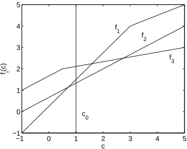
with a varying right-hand side parameter c, we see that fi(c) is piecewise linear, concave, and
nondecreasing in c (Bertsimas and Tsitsiklis, 1997). Furthermore, fi(c0) =r∗(qi). Let ∂fi+ be
the right directional derivative of fi at c=c0, and note that ∂fi+ ≥0. From now on, we assume
that the qi have been ordered so that the sequence ∂fi+ is nonincreasing (e.g., as in Figure 3).
To visualize the ordering that we have introduced, consider the set of possible pairs (r,c), given
a fixed q. That is, consider the set M(qi) ={(r,c):∃p∈∆(A)s.t. r=∑a
,bp(a)qi(b)R(a,b),c= ∑a,bp(a)qi(b)C(a,b)}. The set M(qi)is the image of the simplex under a linear transformation, and is therefore a polytope, as illustrated by the triangular areas in Figure 2. The strategy of P2 is to first
play qi such that the p that maximizes the reward (Eq. 9) satisfies Eq. (10) with equality. (Such a
qi results in a set M(qi)like the one shown in Figure 2(b).) After all these qi are played, P2 plays
those qi for which the p that maximizes the reward (Eq. 9) satisfies Eq. (10) with strict inequality,
and∂fi+=0. (Such a qi results in a set M(qi)like the one shown in Figure 2(a).)
Suppose that P1 knows the sequence q1, . . . ,qk (ordered as above) in advance, and that P2
fol-lows the strategy described earlier. We assume that τ is large enough so that we can ignore the
effects of dealing with a finite sample. Let pi be the average of the mixed actions chosen by P1
while player P2 plays qi. We introduce the constraints
ℓ
∑
i=1αi
∑
a,b
pi(a)qi(b)C(a,b)≤c
0
ℓ
∑
i=1−1 0 1 2 3 4 5 −1
0 1 2 3 4 5
c fi
(c)
f 1
f 2
f 3
c 0
Figure 3: An example of functions fi ordered according to∂fi+.
These constraints must be satisfied in order to guarantee that ˆct has negligible probability of
sub-stantially exceeding c0, at the “switching” times from one mixed action to another. If P1 exploits
the knowledge of P2’s strategy to maximize her average reward at time τ, the resulting expected
average reward at timeτwill be the optimal value of the objective function in the following linear
programming problem:
max p1,p2,...,pk
k
∑
i=1αi
∑
a,b
pi(a)qi(b)R(a,b)
s.t.
ℓ
∑
i=1αi
∑
a,b
pi(a)qi(b)C(a,b)≤c0
ℓ
∑
i=1αi, ℓ=1,2, . . . ,k, (11)
pℓ∈∆(A), ℓ=1,2, . . . ,k.
Of course, given the value of∑a,bpi(a)qi(b)C(a,b), to be denoted by ci, player P1 should choose a pi that maximizes rewards, resulting in∑a,bpi(a)qi(b)R(a,b) = f
i(ci). Thus, the above problem can be rewritten as
max c1,...,ck
∑
αifi(ci)
s.t.
ℓ
∑
i=1αici≤c0
ℓ
∑
i=1αi, ℓ=1,2, . . . ,k. (12)
We claim that letting ci=c0, for all i, is an optimal solution to the problem (12). This will then
imply that the optimal value of the objective function for the problem (11) is∑ki=1αifi(c0), which
equals∑ki=1αir∗(qi), which in turn, is bounded above by ˜r(q0)−ε/2. Thus, ˆr
τ<˜r(q0)−ε/2+δ(τ),
where the termδ(τ) incorporates the effects due to the randomness in the process. By repeating
this argument with ever increasing values of τ (so that the stochastic term δ(τ) is averaged out
and becomes negligible), we obtain that the event ˆrt <˜r(q0)−ε/2 will occur infinitely often, and
therefore ˜r is not attainable.
It remains to establish the claimed optimality of (c0, . . . ,c0). Suppose that (c1, . . . ,ck) 6=
the fiimplies that(c0, . . . ,c0)is also an optimal solution. Otherwise, let j be the smallest index for which cj>c0. If∂f+j =0 (as in the case shown in Figure 2(b)) we have that fi(c)is maximized at
c0 for all i≥ j and(c0, . . . ,c0)is optimal. Suppose that∂f+j >0. In order for the constraint (12) to be satisfied, there must exist some index s< j such that cs<c0. Let us perturb this solution
by settingδ=min{αs(c0−cs),αj(cj−c0)}, increasing csto ˜cs=cs+δ/αs, and decreasing cj to ˜
cj=cj−δ/αj. This new solution is clearly feasible. Let∂fs−=limε↓0(fs(c0)−fs(c0−ε))/ε, which
is the left derivative of fs at c0. Using the concavity of fs, and the earlier introduced ordering, we have∂fs−≥∂fs+≥∂f+j . Observe that
fs(c˜s) = fs(cs) +∂fs−δ/αs,
fj(c˜j) =fj(cj)−∂f+j δ/αj,
so thatαsfs(c˜s) +αjfj(c˜j)≥αsfs(cs) +αjfj(cj). Therefore, the new solution must also be optimal,
but has fewer components that differ from c0. By repeating this process, we eventually conclude
that(c0, . . . ,c0)is an optimal solution of (12).
To the best of our knowledge, this is the first tightness result for a performance envelope (the reward-in-hindsight) different than the Bayes envelope, for repeated games. On the other hand, we
note that our proof relies crucially on the assumption of a single constraint (d=1), which allows us
to order the∂fi+.
6. Attaining the Convex Hull Using Calibrated Forecasts
In this section, we consider a specific strategy that attains the convex hull, thus providing a con-structive proof for Theorem 5. The strategy is based on forecasting P2’s action, and playing a best response (in the sense of Eq. 5) against the forecast. The quality of the resulting strategy depends, of course, on the quality of the forecasts; it is well known that calibrated forecasts lead to no-regret strategies in standard repeated matrix games. See Foster and Vohra (1997) and Cesa-Bianchi and Lugosi (2006) for a discussion of calibration and its implications in learning in games. In this section we consider the consequences of calibrated play for repeated games with constraints.
We start with a formal definition of calibrated forecasts and calibrated play, and then show that calibrated play attains rc in the sense of Definition 1.
A forecasting scheme specifies at each stage k a probabilistic forecast qk∈∆(B)of P2’s action
bk. More precisely a (randomized) forecasting scheme is a sequence of maps that associate with
each possible history hk−1 during the first k−1 stages a probability measure µk over∆(B). The
forecast qk∈∆(B)is then selected at random according to the distribution µk. Let us clarify that for
the purposes of this section, the history is defined to include the realized past forecasts. We shall use the following definition of calibrated forecasts.
Definition 9 (Calibrated forecasts) A forecasting scheme is calibrated if for every (Borel measur-able) set Q⊂∆(B)and every strategy of P1 and P2
lim t→∞
1
t
t
∑
τ=1
1{qτ∈Q}(e(bτ)−qτ) =0, a.s., (13)
Calibrated forecasts, as defined above, have been introduced into game theory in Foster and Vohra (1997), and several algorithms have been devised to achieve them (see Cesa-Bianchi and Lugosi, 2006, and references therein). These algorithms typically start with predictions that are restricted to a finite grid, and gradually increase the number of grid points.
The proposed strategy is to let P1 play a best response against P2’s forecasted play while still satisfying the constraints (in expectation, for the single stage game). Formally, we let:
p∗(q) = argmax p∈∆(A)
∑
a,bp(a)q(b)R(a,b)
s.t.
∑
a,b
p(a)q(b)C(a,b)∈T,
where in the case of a non-unique maximum we assume that p∗(q)is uniquely determined by some
tie-breaking rule; this is easily done, while keeping p∗(·) a measurable function. The strategy is
to play pt = p∗(qt), where qt is a calibrated forecast of P2’s actions.4 We call such a strategy a
calibrated strategy.
The following theorem states that a calibrated strategy attains the convex hull.
Theorem 10 Let Assumption 1 hold, and suppose that P1 uses a calibrated strategy. Then, rc is attained with respect to T .
Proof Fixε>0. We need to show that by playing the calibrated strategy, P1 obtains lim inft→∞(ˆrt− rc(qˆt))≥0 and lim supt→∞dist(cˆt,T)≤0, almost surely.
Fix some ε>0. Consider a partition of the simplex ∆(B) to finitely many measurable sets
Q1,Q2, . . . ,Qℓ such that q,q′ ∈Qi implies that kq−q′k ≤ε andkp∗(q)−p∗(q′)k ≤ε. (Such a
partition exists by the compactness of ∆(B) and ∆(A). The measurability of the sets Qi can be
guaranteed because the mapping p∗(·)is measurable.) For each i, let us fix a representative element
qi∈Qi, and let pi=p∗(qi).
Since we have a calibrated forecast, Eq. (13) holds for every Qi, 1≤i≤ℓ. Define Γt(i) =
∑t
τ=11{qτ∈Qi}and assume without loss of generality thatΓt(i)>0 for large t (otherwise, eliminate
those i for whichΓt(i) =0 for all t, and renumber the Qi). To simplify the presentation, we assume
that for every i, and for large enough t, we haveΓt(i)≥εt. (If for some i, and t this condition is
violated, the contribution of such an i in the expressions that follow will be O(ε).) By a law of large numbers for martingales, we have
lim t→∞ cˆt−
1
t
t
∑
τ=1
C(aτ,bτ)
!
=0, a.s.
By definition, we have
1
t
t
∑
τ=1
C(aτ,bτ) =
∑
i Γt(i)
t
∑
a,bC(a,b)1 Γt(i)
t
∑
τ=1
1{qτ∈Qi}1{aτ=a}1{bτ=b}.
Observe that whenever qτ∈Qi, we havepτ−pi
≤ε, where pτ=p∗(qτ)and pi=p∗(qi)because
of the way the sets Qi were constructed. By martingale convergence, the frequency with which a
will be selected whenever qτ∈Qiand bτ=b, will be approximately pi(a). Hence, for all b,
lim sup t→∞
1 Γt(i) t
∑
τ=1
1{qτ∈Qi}1{aτ=a}1{bτ=b} −pi(a) 1 Γt(i)
t
∑
τ=1
1{qτ∈Qi}1{bτ=b}
≤ε,
almost surely. By the calibration property (13) for Q=Qi, and the fact that whenever q,q′∈Qi, we
havekq−q′k ≤ε, we obtain
lim sup t→∞
1 Γt(i) t
∑
τ=1
1{qτ∈Qi}1{bτ=b} −qi(b)
≤ε, a.s.
By combining the above bounds, we obtain
lim t→∞
ˆ
ct−
∑
iΓt(i)
t
∑
a,bC(a,b)pi(a)qi(b)
≤2ε, a.s. (14)
Note that the sum over index i in Eq. (14) is a convex combination (because the coefficients Γt(i)/t sum to 1) of elements of T (because of the definition of pi), and is therefore an element of
T (because T is convex). This establishes that the constraint is asymptotically satisfied within O(ε).
Note that in this argument, wheneverΓt(i)/t<ε, the summand corresponding to i is indeed of order
O(ε)and can be safely ignored, as stated earlier.
Regarding the average reward, an argument similar to the above yields
lim inf
t→∞ ˆrt ≥lim inft→∞
∑
iΓt(i)
t
∑
a,bR(a,b)pi(a)qi(b)−2ε, a.s.
Next, observe that
∑
iΓt(i)
t
∑
a,bR(a,b)pi(a)qi(b) =
∑
i Γt(i)
t r
∗(qi)≥rc
∑
iΓt(i) t q
i,
where the equality is a consequence of the definition of pi, and the inequality follows by the
def-inition of rc as the closed convex hull of r∗. Observe also that the calibration property (13), with
Q=∆(B), implies that
lim t→∞
ˆ
qt− 1
t
t
∑
τ=1
qτ
=0, a.s.
In turn, sinceqτ−qi
≤εfor a fractionΓt(i)/t of the time,
lim sup t→∞
ˆ
qt−
∑
i Γt(i) t q i=lim sup
t→∞
1 t t
∑
τ=1
qτ−
∑
i Γt(i) t q i≤ε, a.s.
Recall that the function rc is continuous, hence uniformly continuous. Thus, there exists some
function g, with limε↓0g(ε) =0, such that when the argument of rcchanges by at mostε, the value
of rc changes by at most g(ε). By combining the preceding results, we obtain
lim inf t→∞ ˆrt≥r
c(qˆ
The above argument involves a fixedε, and a fixed numberℓof sets Qi, and lets t increase to in-finity. As such, it establishes that for anyε>0 the function rc−2ε−g(ε)is attainable with respect to the set Tεdefined by Tε={x|dist(x,T)≤2ε}. Since this is true for everyε>0, we conclude that the calibrated strategy attains rcas claimed.
7. Algorithms
The results in the previous section motivate us to develop algorithms for online learning with con-straints, perhaps based on calibrated forecasts. For practical reasons, we are interested in computa-tionally efficient methods, but there are no known computacomputa-tionally efficient calibrated forecasting algorithms. For this reason, we will consider related heuristics that are similar in spirit, even if they do not have all the desired guarantees.
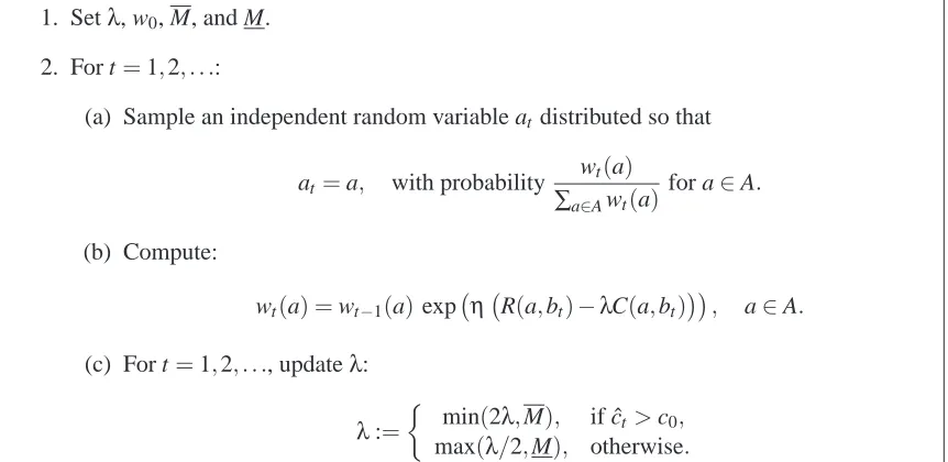
We first consider a method based on the weighted average predictor. The algorithm in Table 1 keeps track of the performance of the different actions in the set A, updating a corresponding set of weights accordingly at each step. The main idea is to quantify “performance” by a linear
com-bination of the total reward and the magnitude of the constraint violation. The parameterλ>0 of
the algorithm, which acts similar to a Lagrange multiplier, determines the tradeoff between these
two objectives. When the average penalty is higher than c0 (i.e., there is a violation), the weight
of the cost term increases. When the average penalty is lower than c0, the weight of the cost term
decreases. The parameters M and M are used to bound the magnitude of the weight of the cost term; in the experiments reported in Section 8, they were set to 1000 and 0.001, respectively.
1. Setλ, w0, M, and M.
2. For t=1,2, . . .:
(a) Sample an independent random variable at distributed so that
at =a, with probability
wt(a) ∑a∈Awt(a)
for a∈A.
(b) Compute:
wt(a) =wt−1(a) exp η R(a,bt)−λC(a,bt)
, a∈A.
(c) For t=1,2, . . ., updateλ:
λ:=
min(2λ,M), if ˆct>c0,
max(λ/2,M), otherwise.
Table 1: Exponentially weighted average predictor.
cases where it is calibrated, in particular if the sequence it tries to calibrate comes from a source with some specific properties; see Mannor et al. (2007) for details. The algorithm is presented in Table 2. If there is a current violation, it selects an action that minimizes the immediate forecasted cost. If the current average penalty does not violate the constraint, it selects a best response to the forecasted action of P2, while satisfying the constraints.
1. Setρ∈(0,1), c0, and f0= (1/|B|)~1.
2. For t=1,2, . . .:
(a) If t=1 or ˆct >c0, choose an action that minimizes the worst-case cost:
at ∈argmin
a∈A
(C(a,b)ft−1(b)),
(b) Otherwise (if ˆct≤c0and t>1), solve
max
p∈∆(A)
∑
a,bp(a)R(a,b)ft−1(b),subject to
∑
a,b
p(a)C(a,b)ft−1(b)≤c0.
and choose a random action distributed according to the solution to the above linear program.
(c) After observing bt, update the forecast ft on the probability distribution of the next
opponent action bt+1:
ft= ft−1+ (1/t)ρ(ebt−ft−1),
where ebis a unit vector inR|B|with the element 1 in the component corresponding
to b∈B.
Table 2: Tracking forecaster.
8. Experimental Setup
However, saving energy by putting the processor in the low-power state comes at a cost. In the low-power state, a delay is incurred each time that the processor moves back into the high-power state in response to user-generated interrupts. We wish to limit the delay perceived by the human user. For this purpose, we assign a cost to the event that an interrupt arrives while the processor is in the low-power state, and impose a constraint on the time average of these costs. A similar model was used in Kveton et al. (2008), and we refer the reader to that work for further details.
We formulate the problem as follows. We divide a typical 16 millisecond interval into ten intervals. We let P1’s action set be A={0,0.1,0.2, . . . ,1}, where action a corresponds to turning
off the CPU after 16a milliseconds (the action a=1 means the CPU is not turned off during the
interval while the action a=0 means it is turned off for the whole interval). Similarly, the action set
of P2 is B={0,0.1,0.2, . . . ,0.9}, where action b corresponds to an interrupt after 16b milliseconds.
(Note that the action b=0 means there is no interrupt and that there is no point in including an
action b=1 in B since it would coincide with the known periodic interrupt.) The assumption is that
an interrupt is handled instantaneously so if the CPU chooses a slightly larger than b it maximizes the power savings while incurring no penalty for observed delay (it is assumed for the sake of discussion that only a single interrupt is possible in each 16 millisecond interval). We define the reward at each stage as follows:
R(a,b) =
1−a, if b=0 or a>b, that is, if no interrupt occurs or an interrupt occurs
before the CPU turns off,
b−a, if b>0 and a≤b, that is, if there is an interrupt
after the CPU is turned off.
The cost is:
C(a,b) =
(
1, if a≤b and b>0,
0, otherwise.
In “normal” operation where the CPU is powered throughout, the action is a=1 and in that case
there is no reward (no power saving) and no cost (no perceived delay). When a=0 the CPU is
turned off immediately and in this case the reward will be proportional to the amount of time until
an interrupt (or until the next decision). The cost in the case a=0 is 0 only is there is no interrupt
(b=0).
We used the real data trace obtained from what is known as MobileMark 2005 (MM05), a performance benchmark that simulates the activity of an average Microsoft Windows user. This CPU activity trace is 90 minutes long and contains more than 500,000 interrupts, including the periodic scheduled interrupts mentioned earlier. The exponentially weighted algorithm (Table 1) and the tracking forecaster (Table 2) were run on this data set. Figure 4 shows the performance of the two algorithms. The straight line shows the tradeoff between constraint violation and average reward by picking a fixed action over the entire time horizon. The different points for the exponential weighted predictor (Table 1) or the tracking forecaster (Table 2) correspond to different values of
c0. We observe that for the same average cost, the tracking forecast performs better (i.e., gets higher
reward).
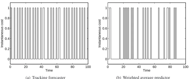
We selected c0=0.3 and used both algorithms for the MM05 trace. Figures 5(a) and 5(b) show
0 0.2 0.4 0.6 0.8 1 0
0.2 0.4 0.6 0.8 1
A
ve
ra
g
e
re
w
a
rd
Average cost Constant actions Tracking forecaster Weighted predictor
Figure 4: Plot of average reward against constraint violation frequency from experiments in power management for the MM05 data.
0 20 40 60 80 100
0 0.2 0.4 0.6 0.8 1
Instantaneous cost
Time
(a) Tracking forecaster
0 20 40 60 80 100
0 0.2 0.4 0.6 0.8 1
Instantaneous cost
Time
(b) Weighted average predictor
Figure 5: Instantaneous cost incurred by the tracking forecaster and weighted average predictor
with target constraint c0=0.3 for the MM05 data.
average reward and average cost for the same experiment. In spite of not being calibrated, the tracking forecast based algorithm outperforms the exponentially weighted based algorithm.
9. Conclusions
0 2 4 6 8 10 0
0.1 0.2 0.3 0.4 0.5
Average reward and cost
Time
Average cost Average reward
(a) Tracking forecaster
0 2 4 6 8 10
0 0.1 0.2 0.3 0.4 0.5
Average reward and cost
Time Average cost Average reward
(b) Weighted average predictor
Figure 6: Time evolution of average reward and average cost for the tracking forecaster and
weighted average forecaster with c0=0.3 for the MM05 data.
we are not aware of any approximate calibration algorithm with comparable convergence rates. Second, the complexity of these two online learning algorithms leaves much to be desired. The complexity of a policy based on approachability theory is left undetermined because we do not have a specific procedure for computing P1’s action at each stage. The per stage complexity is unknown for calibrated forecasts, but is exponential for approximately calibrated schemes (Cesa-Bianchi and Lugosi, 2006). Moreover, it is not clear whether online learning with constraints is as hard computationally as finding a calibrated forecast. Third, we only established the tightness of the lower convex hull of the Bayes envelope for the case of a one-dimensional penalty function. This is a remarkable result because it establishes the tightness of an envelope other than the Bayes envelope, and we are not aware of any such results for similar settings. However, it is not clear whether such a result also holds for two-dimensional penalties. In particular, the proof technique of the tightness result does not seem to extend to higher dimensions.
Our formulation of the learning problem (learning with pathwise constraints) is only a first step in considering multi-objective problems in online learning. In particular, other formulations, for example, that consider the number of time-windows where the constraints are violated, are of interest; see Kveton et al. (2008).
Acknowledgments
References
E. Altman. Constrained Markov Decision Processes. Chapman and Hall, 1999.
D. Bertsimas and J. N. Tsitsiklis. Introduction to Linear Optimization. Athena Scientific, 1997.
D. Blackwell. An analog of the minimax theorem for vector payoffs. Pacific J. Math., 6(1):1–8, 1956a.
D. Blackwell. Controlled random walks. In Proc. Int. Congress of Mathematicians 1954, volume 3, pages 336–338. North Holland, Amsterdam, 1956b.
N. Cesa-Bianchi and G. Lugosi. Prediction, Learning, and Games. Cambridge University Press, 2006.
D. P. Foster and R. V. Vohra. Calibrated learning and correlated equilibrium. Games and Economic
Behavior, 21:40–55, 1997.
J. Hannan. Approximation to Bayes Risk in Repeated Play, volume III of Contribution to The Theory
of Games, pages 97–139. Princeton University Press, 1957.
E. Hazan and N. Megiddo. Online learning with prior information. In Proceedings of 20th Annual
Conference on Learning Theory, 2007.
B. Kveton, J.Y. Yu, G. Theocharous, and S. Mannor. Online learning with expert advice and finite-horizon constraints. In AAAI 2008, in press, 2008.
S. Mannor and N. Shimkin. The empirical Bayes envelope and regret minimization in competitive Markov decision processes. Mathematics of Operations Research, 28(2):327–345, 2003.
S. Mannor and N. Shimkin. A geometric approach to multi-criterion reinforcement learning.
Jour-nal of Machine Learning Research, 5:325–360, 2004.
S. Mannor, J. S. Shamma, and G. Arslan. Online calibrated forecasts: Memory efficiency versus universality for learning in games. Machine Learning, 67(1–2):77–115, 2007.
J. F. Mertens, S. Sorin, and S. Zamir. Repeated games. CORE Reprint Dps 9420, 9421 and 9422, Center for Operation Research and Econometrics, Universite Catholique De Louvain, Belgium, 1994.
N. Shimkin. Stochastic games with average cost constraints. In T. Basar and A. Haurie, editors,
Advances in Dynamic Games and Applications, pages 219–230. Birkhauser, 1994.
X. Spinat. A necessary and sufficient condition for approachability. Mathematics of Operations
Research, 27(1):31–44, 2002.
M. Zinkevich. Online convex programming and generalized infinitesimal gradient ascent. In