Security Analysis of Online Centroid Anomaly Detection
Marius Kloft∗ KLOFT@TU-BERLIN.DE
Machine Learing Group Technische Universit¨at Berlin Franklinstr. 28/29
10587 Berlin, Germany
Pavel Laskov PAVEL.LASKOV@UNI-TUEBINGEN.DE
Wilhelm-Schickard Institute for Computer Science University of T¨ubingen
Sand 1
72076 T¨ubingen, Germany
Editor:Ingo Steinwart
Abstract
Security issues are crucial in a number of machine learning applications, especially in scenar-ios dealing with human activity rather than natural phenomena (e.g., information ranking, spam detection, malware detection, etc.). In such cases, learning algorithms may have to cope with ma-nipulated data aimed at hampering decision making. Although some previous work addressed the issue of handling malicious data in the context of supervised learning, very little is known about the behavior of anomaly detection methods in such scenarios. In this contribution,1 we analyze the performance of a particular method—online centroid anomaly detection—in the presence of adversarial noise. Our analysis addresses the following security-related issues: formalization of learning and attack processes, derivation of an optimal attack, and analysis of attack efficiency and limitations. We derive bounds on the effectiveness of a poisoning attack against centroid anomaly detection under different conditions: attacker’s full or limited control over the traffic and bounded false positive rate. Our bounds show that whereas a poisoning attack can be effectively staged in the unconstrained case, it can be made arbitrarily difficult (a strict upper bound on the attacker’s gain) if external constraints are properly used. Our experimental evaluation, carried out on real traces of HTTP and exploit traffic, confirms the tightness of our theoretical bounds and the practicality of our protection mechanisms.
Keywords: anomaly detection, adversarial, security analysis, support vector data description, computer security, network intrusion detection
1. Introduction
Machine learning methods have been instrumental in enabling novel data analysis applications. Nu-merous currently indispensable technologies—object recognition, user preference analysis, spam filtering, to name only a few—rely on accurate analysis of massive amounts of data. Unfortunately, the increasinguse of machine learning methods gives rise to a threat of theirabuse. A
convinc-∗. MK is also with Department of Brain and Cognitive Engineering, Korea University, Anam-dong, Seongbuk-gu, Seoul 136-713, Korea. Parts of the work were done while MK was with Computer Science Division and Department of Statistics, University of California, Berkeley, CA 94720-1758, USA.
ing example of this phenomenon are emails that bypass spam protection tools. Abuse of machine learning can take on various forms. A malicious party may affect the training data, for example, when it is gathered from the real operation of a system and cannot be manually verified. Another possibility is to manipulate objects observed by a deployed learning system (test data) so as to bias its decisions in favor of an attacker. Yet another way to defeat a learning system is to send a large amount of nonsense data in order to produce an unacceptable number of false alarms and hence force the system’s operator to turn it off. Manipulation of a learning system may thus range from simple cheating to complete disruption of its operation.
A potential insecurity of machine learning methods stems from the fact that they are usually not designed with adversarial input in mind. Starting from the mainstream computational learning theory (Vapnik, 1998; Sch¨olkopf and Smola, 2002), a prevalent assumption is that training and test data are generated from the same fixed, but unknown, probability distribution. This assumption obviously does not hold for adversarial scenarios. Furthermore, even the recent work on learning with non-i.i.d. data (Steinwart et al., 2009; Mohri and Rostamizadeh, 2010) or differing training and test distributions (Sugiyama et al., 2007) is not necessarily appropriate for adversarial input, because in the latter case one must account for a specific worst-case difference while all the aforementioned papers assume that the data is generated stochastically.
Computer security is the most important application field in which robustness of learning algo-rithms against adversarial input is crucial. Modern security infrastructures are facing an increasing professionalization of attacks motivated by monetary profit. A widespread deployment of evasion techniques, such as encryption, obfuscation and polymorphism, is manifested in a rapidly increas-ing diversity of malicious software observed by security experts. Machine learnincreas-ing methods offer a powerful tool to counter a rapid evolution of security threats. For example, anomaly detection can identify unusual events that potentially contain novel, previously unseen exploits (Wang and Stolfo, 2004; Rieck and Laskov, 2006; Wang et al., 2006; Rieck and Laskov, 2007). Another typical ap-plication of learning methods is automatic signature generation which drastically reduces the time needed for development and deployment of attack signatures (Newsome et al., 2006; Li et al., 2006). Machine learning methods can also help researchers better understand the design of malicious soft-ware by using classification or clustering techniques together with special malsoft-ware acquisition and monitoring tools (Bailey et al., 2007; Rieck et al., 2008).
In order for machine learning methods to be successful in security applications—and in gen-eral in any application where adversarial input may be encountered—they should be equipped with countermeasures against potential attacks. The current understanding of security properties of learn-ing algorithms is rather incomplete. Earlier work in the PAC-framework addressed some scenarios in which training data is deliberately corrupted (Angluin and Laird, 1988; Littlestone, 1988; Kearns and Li, 1993; Auer, 1997; Bschouty et al., 1999). These results, however, are not connected to mod-ern learning algorithms used in classification, regression and anomaly detection problems. Several examples of effective attacks were demonstrated in the context of specific security and spam detec-tion applicadetec-tions (Lowd and Meek, 2005a; Fogla et al., 2006; Fogla and Lee, 2006; Perdisci et al., 2006; Newsome et al., 2006; Nelson et al., 2008), which motivated a recent work on taxonomiza-tion of such attacks (Barreno et al., 2006, 2008, 2010). However, it remains largely unclear whether machine learning methods can be protected against adversarial impact.
a theoretical analysis of machine learning algorithms for adversarial scenarios is indispensable. It is hard to imagine, however, that such an analysis can offer meaningful results for any attack in every circumstance. Hence, to be a useful guide for practical applications of machine learning in adversarial environments, such an analysis must address specific attacks against specific learning algorithms. This is precisely the approach followed in this contribution.
The main focus of our work is the security analysis of online centroid anomaly detection against the so-called “poisoning” attacks. Centroid anomaly detection is a very simple method which has been widely used in computer security applications (e.g., Forrest et al., 1996; Warrender et al., 1999; Wang and Stolfo, 2004; Rieck and Laskov, 2006; Wang et al., 2006; Rieck and Laskov, 2007). In the learning phase, centroid anomaly detection computes the mean of all training data points:
c=1
n
n
∑
j=1xj.
Detection is carried out by computing the distance of a new example x from the centroid c and comparing it with an appropriate threshold:
f(x) = (
1, if||x−c||>θ
0, otherwise .
Notice that all operations can be carried out using kernel functions—a standard trick known since the development of support vector machines and kernel PCA (Boser et al., 1992; Sch¨olkopf et al., 1998; Sch¨olkopf and Smola, 2002; Shawe-Taylor and Cristianini, 2004), which substantially increases the discriminative power of this method.
More often than not, anomaly detection algorithms are deployed in non-stationary environments and need to be regularly re-trained. Since the data is fed into the learning phase without any verifica-tion, an adversary has an opportunity to force a learning algorithm to learn a representation suitable for him. One particular kind of attack is the so-called “poisoning” in which specially crafted data points are injected to cause the decision function to misclassify a given malicious point as benign. This attack makes sense when an attacker does not have “write” permission to the training data, hence cannot manipulate it directly. Therefore, his goal is to trick an algorithm by merely using an “append” permission, by sending new data that looks innocuous to the learning algorithm but changes the algorithm’s state in a way that favors the attacker; for example, forcing the algorithm to accept a specific attack point later during the testing stage.
The poisoning attack against online centroid anomaly detection has been considered by Nelson and Joseph (2006) for the case of an infinite window, that is, when a learning algorithm memorizes all data seen so far. Their main result was surprisingly optimistic: it was shown that the number of attack data points that must be injected grows exponentially as a function of the impact over a learned hypothesis. However, the assumption of an infinite window also hinders the ability of a learning algorithm to adjust to legitimate changes in the data distribution.
1.1 Contributions of This Work
using only a linear amount of injected data unless additional constraints are imposed. As a further contribution, we analyze the algorithm under two additional constraints: (a) the fraction of the traffic controlled by an attacker is bounded byν, and (b) the false positive rate induced by an attack is bounded byα. Both constraints can be motivated by an operational practice of anomaly detection systems. Overall, we significantly extend the analysis of Nelson and Joseph (2006) by considering a more realistic learning scenario, explicitly treating potential constraints on the attacker’s part and providing tighter bounds.
Our analysis methodology follows the following framework, which can be used for any kind of quantitative security analysisof learning algorithms (Laskov and Kloft, 2009):
1. Axiomatic formalization of the learning and the attack processes. Such a formalization in-cludes definitions of data sources and objective (risk) functions used by each party, as well as the attacker’s goal. It specifies the knowledge available to an attacker, that is, whether he knows an algorithm, its parameters and internal state, and which data he can potentially manipulate.
2. Specification of an attacker’s constraints. Potential constraints on the attacker’s part may in-clude: percentage of traffic under his control, amount of additional data that must be injected, an upper bound on the norm of a manipulated part, a maximal allowable false-positive rate (in case an attack must be stealthy), etc. Such constraints must be incorporated into the axiomatic formalization.
3. Investigation of the optimal attack policy. Such a policy may be long-term; that is, over multiple attack iterations, as well as short-term, for a single iteration. The investigation can be carried out either as a formal proof or numerically, by casting the search for an attack policy as an optimization problem.
4. Bounding the attacker’s gain under the optimal policy. The ultimate goal of our analysis is to quantify the attacker’s gain or effort under his optimal policy. Such an analysis may take different forms, for example calculation of the probability for an attack to succeed, estimation of the required number of attack iterations, calculation of the geometric impact of an attack (a shift towards an insecure state), etc.
r centroid’s radius
i attack iteration index,i∈N0
ci center of centroid ini-th attack iteration
A attack point
a attack direction vector
Di i-th relative displacement of a centroid in radii
into direction ofa
n number of patterns used for initial training of the centroid
f attack strategy function
ν fraction of adversarial training points Bi Bernoulli random variable
xi training data α false alarm rate
IS indicator function of a setS
Table 1: Notation summary.
1.2 Poisoning and Related Attacks Against Learning Algorithms
For two-class learning problems, attacks against learning algorithms can be generally classified according to the following two criteria (the terminology in the taxonomy of Barreno et al. (2006) is given in brackets):
• whether an attack is staged during the training (causative) or the deployment of an algorithm (exploratory), or
• whether an attack attempts to increase the false negative or the false positive rate at the de-ployment stage (integrity/availability).
The poisoning attack addressed in our work can be classified as a causative integrity attack. This scenario is quite natural, for example, in web application scenarios in which the data on a server can be assumed to be secure but the subsequent injection of adversarial data cannot be easily prevented. Other common attack types are the mimicry attack—alteration of malicious data to resemble in-nocuous data (an exploratory integrity attack) and the “red herring” attack—sending junk data that causes false alarms (an exploratory availability attack). Attacks of the latter two kinds are beyond the scope of our investigation.
approxi-mately the same innocuous data the algorithm is trained on. Hence, we will assume that the attacker has precise knowledge of the trained model throughout the attack.
2. Learning and Attack Models
Before proceeding with the analysis, we first present the precise models of the learning and the attack processes.
2.1 Centroid Anomaly Detection
Given a data setX0={x( 1) 0 , . . . ,x
(n)
0 } ⊂Rd, the goal of anomaly detection (also often referred to as “novelty detection”) is to determine whether an example xis unlikely to have been generated by the same distribution as the setX0. A natural way to perform anomaly detection is to estimate the probability density function of the distribution from which the set X0 was drawn and markx as anomalous if it comes from a region with low density. In general, however, density estimation is a difficult problem, especially in high dimensions. A large amount of data is usually needed to reliably estimate the density in all regions of the space. For anomaly detection, knowing the density in the entire space is superfluous, as we are only interested in deciding whether a specific point lies within a “sparsely populated” area. Hence several direct methods have been proposed for anomaly detection, for example, one-class SVM (Sch¨olkopf et al., 2001), support vector data description (SVDD) (Tax and Duin, 1999a,b), and density level set estimation (Polonik, 1995; Tsybakov, 1997; Steinwart et al., 2005). A comprehensive survey of anomaly detection techniques can be found in Markou and Singh (2003a,b).
In the centroid anomaly detection, an Euclidean distance from the empirical mean of the data is used as a measure of abnormality:
f(x) =||x−1
n
n
∑
j=1x(0j)||.
If a hard decision is desired instead of a soft abnormality score, the data point is considered anoma-lous if its score exceeds a fixed thresholdr.
Despite its straightforwardness, a centroid model can represent complex density level sets us-ing a kernel mappus-ing (M¨uller et al., 2001; Sch¨olkopf and Smola, 2002) (see Figure 1). Centroid anomaly detection can be seen as a special case of the SVDD with outlier fraction η=1 and of the Parzen window density estimator (Parzen, 1962) with Gaussian kernel function k(x,y) =
1
(√2πσ)dexp(− 1
2σ2kx−yk2).
Figure 1: Illustration of the density level estimation using a centroid model with a non-linear kernel.
2.2 Online Anomaly Detection
The majority of anomaly detection applications have to deal with non-stationary data. This is espe-cially typical for computer security, as the processes being monitored usually change over time. For example, network traffic characteristics are strongly influenced by the time of the day; system call sequences depend on the applications running on a computer. The model of normality constructed by anomaly detection algorithms hence needs to be regularly updated, in the extreme case—after the arrival of each data point. Obviously, retraining the model from scratch every time is computa-tionally inefficient; however, the incorporation of new data points and the removal of irrelevant ones can be done with acceptable effort (e.g., Laskov et al., 2006).
For centroid anomaly detection, we assume that the initial state of the learner comprises a center c0and a given radiusr. We further assume that this state has been obtained from purely innocuous data. Whenever a new data point xi arrives at iteration i∈N, the learner’s center of mass ci is
updated if and only if the new data point is considered non-anomalous; otherwise, it is rejected and not used for re-training. The radiusrstays fixed over time.2 Recalculation of the center of mass is straightforward and requiresO(1)work. If all examples are “memorized”, that is,Xi=Xi−1∪{xi},3
the update is computed as
ci+1=
1− 1 n+i
ci+
1
n+ixi. (1)
For a finite horizon, that is,∀i:|Xi|=n, in each iterationi, some previous examplexold∈Xiis
replaced by the newly arrivingxi, and the update is thus performed as
ci+1=ci+
1
n(xi−xold). (2)
The update formula can be generalized toci+1=ci+κi(xi−xold), with fixedκ≥0. This changes the bounds in the upcoming analysis only by a constant factor in this case, which is negligible.
2. From the operational standpoint, this assumption is reasonable as the radius serves as a threshold and is usually set and manually tuned after inspection of (false) alarms. Treating the radius as a model parameter would necessitate complex rules for its update and would open the system to poisoning attacks against the radius.
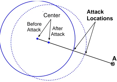
A
Attack Locations
Before
Attack After Attack
Center
Figure 2: Illustration of a poisoning attack. By iteratively inserting malicious training points an attacker can gradually “drag” the centroid into a direction of an attack. The radius is assumed to stay fixed over time. Figure taken from Nelson and Joseph (2006).
Various strategies can be used to determine the “least relevant” pointxold to be removed from the working set:
(a) oldest-out: the point with the oldest timestamp is removed.
(b) random-out: a randomly chosen point is removed.
(c) nearest-out: the nearest-neighbor of the new pointxis removed.
(d) average-out: the center of mass is removed. The new center of mass is recalculated asci+1= ci+1n(xi−ci), which is equivalent to Equation (1) with constantn.
The strategies (a)–(c) require the storage of all points in the working set, whereas the strategy (d) can be implemented by holding only the center of mass in memory.
2.3 Poisoning Attack
The goal of a poisoning attack is to force an algorithm, at some learning iterationi, to accept the attack pointAthat lies outside of the normality ball, that is,||A−ci||>r. It is assumed that the
attacker knows the anomaly detection algorithm and the training data. Furthermore, the attacker cannot modify any existing data except for adding new points. Although the attacker can send any data point, it obviously only makes sense for him to send points lying within the current sphere as they are otherwise discarded by the learning algorithm. As illustrated in Figure 2, the poisoning attack amounts to injecting specially crafted points that are accepted as innocuous but shift the center of mass in the direction of the attack point until the latter appears innocuous as well.
What points should be used by an attacker in order to subvert online anomaly detection? Intu-itively, one can expect that the optimal one-step displacement of the center of mass is achieved by placing attack pointxi along the line connectingc andAsuch that||xi−c||=r. A formal proof
Definition 1 (Relative displacement) LetAbe an attack point anda= A−c0
||A−c0|| be the attack
di-rection unit vector. The i-th relative displacementDiof an online centroid learner is defined as
Di=
(ci−c0)·a
r .
The relative displacement measures the length of the projection of accrued change tocionto the
attack directionain terms of the radius of the normality ball. Note that the displacement is a relative quantity, that is, we may without loss of generality translate the coordinate system so that the center of mass lies at the origin (i.e.,c0=0) and subsequently isotropically normalize the space so that the centroid has unit radiusr=1. After this transformation, the formula for the displacement can be simplified to
Di=ci·a.
Definition 2 An attack strategy that maximizes the displacement Diin each iteration i is referred to
asgreedy-optimal.
3. Attack Effectiveness for Infinite Horizon Centroid Learner
The effectiveness of a poisoning attack for the infinite horizon learner has been analyzed in Nelson and Joseph (2006). We provide an alternative proof that follows the main steps of the framework proposed in Section 1.1.
Theorem 3 The i-th relative displacement Diof the online centroid learner with an infinite horizon
under a poisoning attack is bounded by
Di≤ln
1+i
n
, (3)
where i is the number of attack points and n is the number of initial training points.
Proof We first determine the greedy-optimal attack strategy and then bound the attack progress. (a) Let A be an attack point and denote bya the corresponding attack direction vector. Let
{xi|i∈N} be adversarial training points. The center of mass at the ith iteration is given in the
following recursion:
ci+1=
1− 1 n+i
ci+
1
n+ixi+1, (4)
with initial value c0 =0. By the construction of the poisoning attack, ||xi−ci|| ≤r, which is
equivalent toxi=ci+biwith||bi|| ≤r. Equation (4) can thus be transformed into
ci+1=ci+
1 n+ibi.
Taking the scalar product withaand using the definition of a relative displacement, we obtain:
Di+1=Di+
1 n+i·
bi·a
withD0=0. The right-hand side of the Equation (5) is clearly maximized under||bi|| ≤1 by setting
bi=ra. Thus the greedy-optimal attack is given by
xi=ci+ra. (6)
(b) Plugging the optimal strategybi=rainto Equation (5), we obtain:
Di+1=Di+
1 n+i.
This recursion can be explicitly solved, taking into account thatD0=0, resulting in:
Di= i
∑
k=11 n+k =
n+i
∑
k=11 k−
n
∑
k=11 k.
Inserting the upper bound on the harmonic series,∑mk=11k =ln(m) +εm, withεm≥0, into the above
formula and noting thatεmis monotonically decreasing, we obtain:
Di≤ln(n+i)−ln(n) =ln
n+i n
=ln
1+ i
n
,
which completes the proof.
Since the bound in Equation (3) is monotonically increasing, we can invert it to obtain a bound on the effort needed by an attacker to achieve his goal:
i≥n·(exp(Di)−1).
It can be seen that the effort needed to poison an online centroid learner isexponentialin terms of the relative displacement of the center of mass.4 In other words, an attacker’s effort grows prohibitively fast with respect to the separability of the attack from innocuous data. For a kernelized centroid learner, the greedy-optimal attack may not be valid, as there may not exist a point in the input space corresponding to the optimal attack image in the feature space. However, an attacker can construct points in the input space that are close enough to the greedy-optimal point for the attack to succeed, with a moderate constant cost factor; cf., Section 8.5.
4. Poisoning Attack against Finite Horizon Centroid Learner
The optimistic result presented in Section 3 is unfortunately not quite useful. In practice, memo-rization of all training points essentially defeats the main purpose of an online algorithm, that is, its ability to adjust to non-stationarity. Hence it is important to understand how the removal of data points from the working set affects the security of online anomaly detection. To this end, the spe-cific removal strategies presented in Section 2.2 must be considered. The analysis can be carried out theoretically for the average-out and random-out update rules; for the nearest-out rule, an op-timal attack can be stated as an optimization problem and the attack effectiveness can be analyzed empirically.
4.1 Poisoning Attack for Average-out, Random-out and Oldest-out Rules
We begin our analysis with the average-out learner which follows exactly the same update rule as the infinite-horizon online centroid learner with the exception that the window sizenremains fixed instead of growing indefinitely (cf. Section 2.2). Despite the similarity to the infinite-horizon case, the result presented in the following theorem is surprisingly pessimistic.
Theorem 4 The i-th relative displacement Di of the online centroid learner with the average-out
update rule under a worst-case optimal poisoning attack is
Di=
i n,
where i is the number of attack points and n is the training window size.
Proof The proof is similar to the proof of Theorem 3. By explicitly writing out the recurrence between subsequent displacements, we conclude that the greedy-optimal attack is also attained by placing an attack point along the line connectingciandAat the edge of the sphere (cf. Equation (6)):
xi=ci+ra.
It follows that the relative displacement under the greedy-optimal attack is
Di+1=Di+
1 n.
Since this recurrence is independent of the running indexi, the displacement is simply accumulated over each iteration, which yields the bound of the theorem.
One can see that, unlike the logarithmic bound in Theorem 3, the average-out learner is charac-terized by a linear bound on the displacement. As a result, an attacker only needs a linear number of injected points—instead of an exponential one—in order to subvert an average-out learner. This cannot be considered secure.
A similar result, in terms of theexpectationof the relative displacement, can be obtained for the random-out removal strategy. The proof is based on the observation that in expectation, the average-out rule is equivalent to the random-average-out rule. The oldest-average-out rule can also be handled similarly to the average-out rule by observing that in both cases some fixed point known in advance is removed from a working set, which allows an attacker to easily find an optimal attack point.
4.2 Poisoning Attack for Nearest-out Rule
4.2.1 GREEDY-OPTIMALATTACK
Thegreedy-optimalattack should provide a maximal gain for an attacker in a single iteration. For the infinite-horizon learner (and hence also for the average-out learner, as it uses the same recurrence in a proof), it is possible to show that the greedy-optimal attack yields the maximum gain for the entire sequence of attack iterations; that is, it is (globally) optimal. For the nearest-out learner, it is hard to analyze the full sequence of attack iterations, hence we limit our analysis to a single-iteration gain. Empirically, even a greedy-optimal attack turns out to be effective.
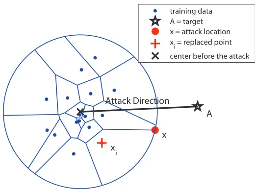
To construct a greedy-optimal attack, we partition the sphere spanned by the centroid into Voronoi cellsVj centered at the training data pointsxj, j=1, . . . ,n. Each Voronoi cell comprises
points for whichxj is the nearest neighbor. Whenever a new training point “falls into” the sphere,
the center of the corresponding Voronoi cell is removed according to the nearest-out rule.
The optimal attack strategy is now straightforward. First, we determine the optimal attack loca-tion within each cell. This can be done by solving the following optimizaloca-tion problem for a fixed xj:
Optimization Problem 5 (greedy-optimal attack)
x∗j = argmax x
yj(x):= (x−xj)·a (7)
s.t. kx−xjk ≤ kx−xkk, ∀k=1, ...,n (8)
kx−1n∑nk=1xkk ≤r. (9)
The objective of the optimization problem (7) reflects the goal of maximizing the projection ofx−xj
onto the attack directiona. The constraint (8) stipulates that the pointxj is the nearest neighbor of
x. The constraint (9), when active, enforces that no solution lies outside of the sphere.
The geometry of the greedy-optimal attack is illustrated in Figure 3. An optimal attack point is placed at the “corner” of a Voronoi cell (including possibly a round boundary of the centroid) to cause the largest displacement of the centroid along the attack direction.
Once the candidate attack locations are found for each of thenVoronoi cells, the one that has the highest value of the objective function yj(x∗j) is injected and the respective centerxj∗ of the Voronoi cell is expunged from the training set:
j∗=argmaxj∈1,...,nyj(x∗j). (10)
The optimization problem (7) can be simplified by plugging in the definition of the Euclidean norm. In the resulting optimization problem, all but one of the norm constraints are reduced to simpler linear constraints:
x∗j = argmax x
(x−xj)·a
s.t. 2(xk−xj)·x≤xk·xk−xj·xj, ∀k=1, ...,n (11)
x·x−2n∑kn=1x·xk≤r2−n12∑nk,l=1xk·xl.
A
x
x i
training data A = target x = attack location xi = replaced point
center before the attack
Attack Direction
Figure 3: The geometry of a poisoning attack for the nearest-out rule. A greedy-optimal attack is injected at the boundary of the respective Voronoi cell.
can optimize such quadratically constrained linear programs (QCLP) with high efficiency, espe-cially when there is only a single quadratic constraint. Alternatively, one can use specialized algo-rithms for linear programming with a single quadratic constraint (van de Panne, 1966; Martein and Schaible, 2005) or convert the quadratic constraint to a second-order cone (SOC) constraint and use general-purpose conic optimization methods.
4.2.2 IMPLEMENTATION OF AGREEDY-OPTIMALATTACK
For the practical implementation of the attack specified by problem (11), some additional processing steps must be carried out.
A point can become “immune” to a poisoning attack, if starting from some iterationi′its Voronoi cell does not overlap with the hypersphere of radiusr centered atci′. The quadratic constraint (9) is never satisfied in this case, and the inner optimization problem (7) becomes infeasible. These immune points remain in the working set forever and slow down the attack’s progress. To avoid this situation, an attacker must keep track of all optimal solutionsx∗j of the inner optimization problems. If an online update would cause some Voronoi cellVj to completely slip out of the hypersphere an
attacker should ignore the outer loop decision (10) and expungexj instead ofxj∗.
A significant speedup can be attained by avoiding the solution of unnecessary QCLP problems. LetS={1, . . . ,j−1}andαSbe the current best solution of the outer loop problem (10) over the
setS. LetyαS be the corresponding objective value of an inner optimization problem (11). Consider the following auxiliary quadratic program (QP):
maxx kx−1n∑nk=1xkk (12)
s.t. 2(xk−xj)·x≤xk·xk−xj·xj, ∀k=1, ...,n (13)
Its feasible set comprises the Voronoi cell of xj, defined by constraint (13), further reduced by
constraint (14) to the points that improve the current valueyαS of the global objective function. If the objective function value provided by the solution of the auxiliary QP (12) exceedsr then the solution of the local QCLP (11) does not improve the global objective function yαS. Hence the expensive QCLP optimization can be skipped.
4.2.3 ATTACKEFFECTIVENESS
To evaluate the effectiveness of the greedy-optimal attack, we perform a simulation on artificial geometric data. The goal of this simulation is to investigate the behavior of the relative displacement Diduring the progress of the greedy-optimal attack.
An initial working set of sizen=100 is sampled from ad-dimensional Gaussian distribution with unit covariance (experiments are repeated for various values ofd∈ {2, ...,100}). The radius r of the online centroid learner is chosen such that the expected false positive rate is bounded by
α=0.001. An attack directiona,kak=1, is chosen randomly, and 500 attack iterations (5∗n) are generated using the procedure presented in Sections 4.2.1–4.2.2. The relative displacement of the center in the direction of the attack is measured at each iteration. For statistical significance, the results are averaged over 10 runs.
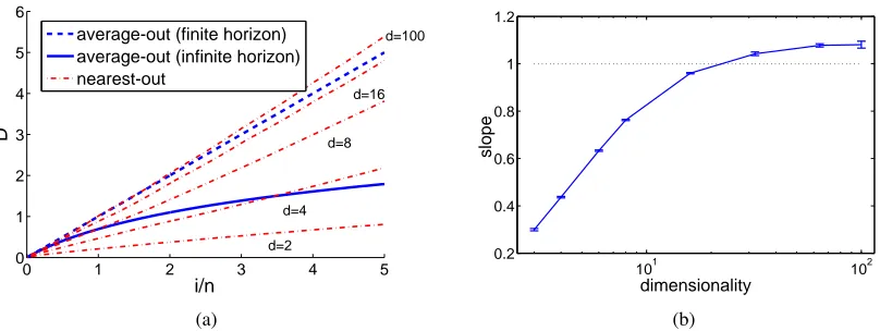
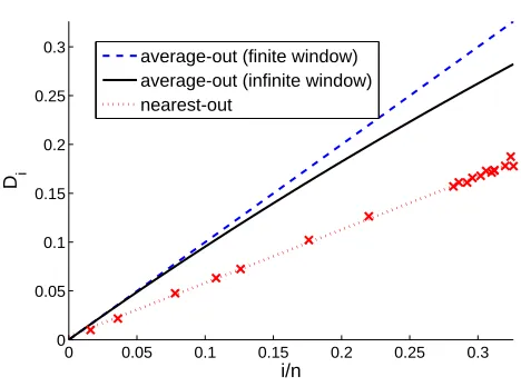
Figure 4(a) shows the observed progress of the greedy-optimal attack against the nearest-out learner and compares it to the behavior of the theoretical bounds for the infinite-horizon learner (the bound of Nelson and Joseph, 2006) and the average-out learner. The attack effectiveness is measured for all three cases by the relative displacement as a function of the number of iterations. Plots for the nearest-out learner are presented for various dimensionsd of the artificial problems tested in simulations. The following observations can be made from the plot provided in Figure 4(a).
First, the attack progress, that is, the functional dependence of the relative displacement of the greedy-optimal attack against the nearest-out learner with respect to the number of iterations, is linear. Hence, contrary to our initial intuition, the removal of nearest neighbors of incoming points does not lead to better security against poisoning attacks.
Second, the slope of the linear attack progressincreases with the dimensionality of the problem. For low dimensionality, the relative displacement of the nearest-out learner is comparable, in abso-lute terms, with that of the infinite-horizon learner. For high dimensionality, the nearest-out learner becomes even less secure than the simple average-out learner. By increasing the dimensionality beyondd>nthe attack effectiveness cannot be increased. Mathematical reasons for this behavior are investigated in Section A.1.
A further illustration of the behavior of the greedy-optimal attack is given in Figure 4(b), show-ing the dependence of the average attack slope on the dimensionality. One can see that the attack slope increases logarithmically with the dimensionality and wanes out to a constant factor after the dimensionality exceeds the number of training data points. A theoretical explanation of the observed experimental results is given in Appendix A.1.2.
4.3 Concluding Remarks
0 1 2 3 4 5 0
1 2 3 4 5 6
i/n
D
average-out (finite horizon) average-out (infinite horizon) nearest-out
d=16
d=8
d=4
d=100
d=2
(a)
101 102
0.2 0.4 0.6 0.8 1 1.2
dimensionality
slope
(b)
Figure 4: Effectiveness of the poisoning attack for the nearest-out rule as a function of input space dimensionality. (a) The displacement of the centroid along the attack direction grows linearly with the number of injected points. Upper bounds on the displacement of the average-out rule are plotted for comparison. (b) The slope of the linear growth increases with the input space dimensionality.
As a compromise, one can in practice choose a large working set sizen, which reduces the slope of a linear attack progress.
Among the different outgoing point selection rules, the nearest-out rule presents the most chal-lenges for the implementation of an optimal attack. Some approximations make such an attack feasible while still maintaining a reasonable progress rate. The key factor for the success of a poi-soning attack in the nearest-out case lies in high dimensionality of the feature space. The progress of an optimal poisoning attack depends on the size of the Voronoi cells induced by the training data points. The size of the Voronoi cells is related linearly to the volume of the sphere corresponding to the attack’s feasible region (see Appendix A.1.2 for a theoretical discussion of this effect). With the increasing dimensionality of the feature space, the volume of the sphere increases exponentially, which leads to a higher attack progress rate.
In the following sections, we analyze two additional factors that affect the progress of a poi-soning attack. First, we consider the case when the attacker controls only a fixed fractionνof the training data. Subsequently we analyze a scenario in which an attacker is not allowed to exceed a certain false positive rateα; for example, by stopping online learning when a high false positive rate is observed. It will be shown that both of these possible constraints significantly reduce the effectiveness of poisoning attacks.
5. Poisoning Attack with Limited Bandwidth Constraint
difficulty of an attack. The choice of realistic values ofνis application-specific. For simplicity, we restrict ourselves to the average-out learner as we have seen that it only differs by a constant from the nearest-out one and is equivalent in expectation to the random-out one.
5.1 Learning and Attack Models
As discussed in Section 2, we assume that the initial online centroid learner is centered at the positionc0 and has a fixed radius r (without loss of generality c0=0 and r=1; cf. discussion after Definition 1 in Section 2). At each iteration a new training point arrives—which is either inserted by an adversary or drawn independently from the distribution of innocuous points—and a new center of mass ci is calculated. The mixing of innocuous and attack points is modeled by a
Bernoulli random variable with the parameterνwhich denotes the probability that an adversarial point is presented to the learner. Adversarial pointsAi are chosen according to the attack function
f depending on the actual state of the learnerci. The innocuous pool is modeled by a probability
distribution from which the innocuous points xi are independently drawn. We assume that the
expectation of innocuous pointsxicoincides with the initial center of mass:E(xi) =c0.
For simplicity, we make one additional assumption in this chapter: all innocuous points are accepted by the learner at any time of the attack independent of their actual distance to the center of mass. In the absence of this assumption, we would need special treatment for the case that a truly innocuous point is disregarded by the learner as the center of mass is getting displaced by the attack. In the next section we drop this assumption so that the learner only accepts points which fall within the actual radius.
The described probabilistic model is formalized by the following axiom.
Axiom 6 {Bi|i∈N} are independent Bernoulli random variables with parameter ν>0. xi are
i.i.d. random variables in a Euclidean space Rd, drawn from a fixed but unknown distribution
Px, satisfying E(x) =0 and kxk ≤r
w.l.o.g.
= 1. Bi and xj are mutually independent for each i,j.
f :Rd →Rd is a functionkf(x)−xk ≤r that we callattack strategy. {ci|i∈N}is a collection of
random vectors such that w.l.o.g.c0=0and ci+1=ci+
1
n(Bif(ci) + (1−Bi)xi−ci). (15)
Moreover, we denote xi:=xi·a.
For simplicity of notation, in this section we refer to a collection of random vectors{ci|i∈N}
satisfying Axiom 6 as anonline centroid learner. Any function f satisfying Axiom 6 is called an attack strategy. The attack strategy is a function that maps a vector (the center) to an attack location. According to the above axiom, the adversary’s attack strategy is formalized by an arbitrary function f. This raises the question of which attack strategies are optimal in the sense that an attacker reaches his goal of concealing a predefined attack direction vector in a minimal number of iterations. As in the previous sections, an attack’s progress is measured by projecting the current center of mass onto the attack direction vector:
Di=ci·a.
Attack strategies maximizing the displacement Di in each iteration i are referred to as
5.2 Greedy-Optimal Attack
The following result characterizes the greedy-optimal attack strategy for the model specified in Axiom 6.
Proposition 7 Letabe an attack direction vector. Then thegreedy-optimal attack strategy f against the online centroid learner is given by
f(ci):=ci+a. (16)
Proof Since by Axiom 6 we have kf(x)−xk ≤r, any valid attack strategy can be written as f(x) =x+g(x), such thatkgk ≤r=1.It follows that
Di+1=ci+1·a
=
ci+
1
n(Bif(ci) + (1−Bi)xi−ci)
·a
=Di+
1
n(BiDi+Big(ci)·a+ (1−Bi)x·a−Di).
SinceBi≥0, the greedy-optimal attack strategy should maximizeg(ci)·asubject to||g(ci)|| ≤1.
The maximum is clearly attained by settingg(ci) =a.
Note that the displacement measures the projection of the change of the centroid onto the attack direction vector. Hence it is not surprising that the optimal attack strategy is independent of the actual position of the learner.
5.3 Attack Effectiveness
The effectiveness of the greedy-optimal attack in the limited control case is characterized in the following theorem.
Theorem 8 For the displacement Diof the centroid learner under an optimal poisoning attack,
(a) E(Di) = (1−ai) ν
1−ν
(b) Var(Di) ≤ γi
ν
1−ν 2
+δn,
where ai:= 1−1−nν i
, bi= 1−1−nν 2−1n i
,γi=ai−bi, andδn:= ν
2+(1
−bi) (2n−1)(1−ν)2.
Proof (a) Inserting the greedy-optimal attack strategy of Equation (16) into Equation (15) of Ax-iom 6, we have:
ci+1=ci+
1
n(Bi(ci+a) + (1−Bi)xi−ci), which can be rewritten as:
ci+1=
1−1−Bi n
ci+
Bi
na+
(1−Bi)
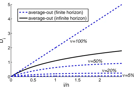
0 0.5 1 1.5 2 0
1 2 3 4 5
i/n
D i
average-out (finite horizon) average-out (infinite horizon)
ν=5% ν=100%
ν=50%
ν=20%
Figure 5: Theoretical behavior of the displacement of a centroid under a poisoning attack for a bounded fraction of traffic under attacker’s control. The infinite horizon bound of Nelson et al. is shown for comparison (solid line).
Taking the expectation on the latter equation and noting that by Axiom 6,E(xi) =0 andE(Bi) =ν, we have
E(ci+1) =
1−1−ν n
E(ci) + ν
na,
which by the definition of the displacement translates to
E(Di+1) =
1−1−ν n
E(Di) + ν
n.
The statement (a) follows from the latter recursive equation by Proposition 17 (formula of the geo-metric series). For the more demanding proof of (b), see Appendix A.2.
The following corollary shows the asymptotic behavior of the above theorem.
Corollary 9 For the displacement Diof the centroid learner under an optimal poisoning attack,
(a) E(Di) ≤ ν
1−ν for all i (b) Var(Di) → 0 for i,n→∞.
Proof The corollary follows from the fact thatγi,δn→0 fori,n→∞.
0 1 2 3 4 5 0
0.01 0.02 0.03 0.04 0.05 0.06
i/n
D i
empirical displacement theoretical displacement
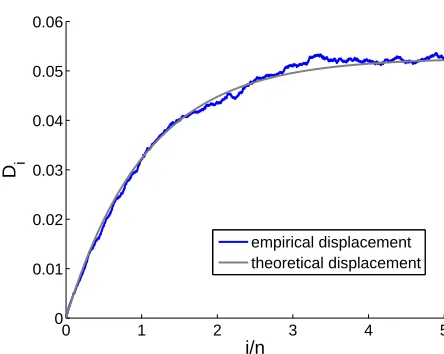
Figure 6: Comparison of the empirical displacement of the centroid under a poisoning attack with attacker’s limited control (ν=0.05) with the theoretical bound for the same setup. The empirical results are averaged over 10 runs.
To empirically investigate the tightness of the derived bound we compute a Monte Carlo simula-tion of the scenario defined in Axiom 6 with the parametersν=0.05,n=100000,
H
=R2, andPxbeing a uniform distribution over the unit circle. Figure 6 shows a typical displacement curve over the first 500,000 attack iterations. One can clearly see that the theoretical bound is closely followed by the empirical simulation.
6. Poisoning Attack under False Positive Constraints
In the last section we have assumed, that innocuous training points xi are always accepted by the
online centroid learner. It may, however, happen that some innocuous points fall outside of the hypersphere boundary while an attacker displaces the hypersphere. We have seen that the attacker’s impact highly depends on the fraction of points he controls. If an attacker succeeds in pushing the hypersphere far enough for innocuous points to start dropping out, the speed of the hypersphere displacement increases. Hence additional protection mechanisms are needed to prevent the success of an attack.
6.1 Learning and Attack Models
Motivated by the above considerations we modify the probabilistic model of the last section as follows. Again we consider the online centroid learner initially anchored at a positionc0 having a radiusr. For the sake of simplicity and without loss of generality we can again assumec0=0 andr=1. Innocuous and adversarial points are mixed into the training data according to a fixed fraction controlled by a binary random variableBi. In contrast to Section 5, innocuous pointsxiare
accepted if and only if they fall within the radiusrfrom the hypersphere’s centerci. In addition, to
innocuous points rejected by the learner, is bounded byα. If the latter is exceeded, we assume the adversary’s attack to have failed and a safe state of the learner to be loaded.
We formalize this probabilistic model as follows:
Axiom 10 {Bi|i∈N}are independent Bernoulli random variables with parameter ν>0. xi are
i.i.d. random variables in a reproducing kernel Hilbert space
H
drawn from a fixed but unknown distribution Px, satisfying E(x) =0, kxk ≤r =1, and Px·a =P−x·a (symmetry w.r.t. the attackdirection). Bi and xj are mutually independent for each i,j. f :Rd →Rd is an attack strategy
satisfyingkf(x)−xk ≤r.{ci|i∈N}is a collection of random vectors such thatc0=0and ci+1=ci+
1
n Bi(f(ci)−ci) + (1−Bi)I{kxi−cik≤r}(xi−ci)
,
if Ex I{kx−cik≤r}
≤1−αand byci+1=0otherwise. Moreover, we denote xi:=xi·a.
For simplicity of notation, we refer to a collection of random vectors{ci|i∈N}satisfying
Ax-iom 10 as anonline centroid learner with maximal false positive rateαin this section. Any function f satisfying Axiom 10 is called an attack strategy. Optimal attack strategies are characterized in terms of the displacement as in the previous sections. Note thatEx(·) denotes the conditional ex-pectation given all remaining random quantities except forx.
The intuition behind the symmetry assumption in Axiom 10 is that it ensures that resetting the centroid’s center to zero (initiated by the false positive protection) does not lead to a positive shift of the centroid toward the attack direction.
6.2 Greedy-Optimal Attack and Attack Effectiveness
The following result characterizes the greedy-optimal attack strategy for the model specified in Axiom 10. We restrict our analysis to greedy-optimal strategies, that is, the ones that maximize the displacement in each successive iteration.
Proposition 11 Letabe an attack direction vector and consider the centroid learner with maximal false positive rateαas defined in Axiom 10. Then thegreedy-optimalattack strategy f is given by
f(ci):=ci+a.
Proof Since by Axiom 10 we have kf(x)−xk ≤r, any valid attack strategy can be written as f(x) =x+g(x), such thatkgk ≤r=1.It follows that eitherDi+1=0, in which case the optimal f is arbitrary, or we have
Di+1 = ci+1·a
=
ci+
1
n(Bif(ci) + (1−Bi)xi−ci)
·a
= Di+
1
n(Bi(Di+g(ci)) + (1−Bi)xi−Di).
SinceBi≥0, the greedy-optimal attack strategy should maximizeg(ci)·asubject to||g(ci)|| ≤1.
The maximum is clearly attained by settingg(ci) =a.
Theorem 12 For the displacement Diof a centroid learner with maximal false positive rateαunder
a poisoning attack,
(a) E(Di) ≤(1−ai)
ν+α(1−ν) (1−ν)(1−α)
(b) Var(Di) ≤γi
ν2
(1−α)2(1−ν)2+ρ(α) +δn, where ai :=
1−(1−ν)(n1−α)i, bi = 1−1−nν(2−1n)(1−α) i
, γi = (ai − bi),
ρ(α) =α(1−ai)(1−bi)(2ν(1−α)+α) (1−1
2n)(1−ν)2(1−α)2
, andδn=(1−bi)(ν+(1−ν)E(xi
2))
(2n−1)(1−ν)(1−α) , xi:=xi·a.
The proof is technically demanding and is given in Appendix A.3. Despite the more general proof reasoning, we recover the tightness of the bounds of the previous section for the special case ofα=0, as shown by the following corollary.
Corollary 13 Suppose a maximal false positive rate ofα=0. Then, the bounds on the expected displacement Di, as given by Theorem 8 and Theorem 12, coincide. Furthermore, the variance
bound of Theorem 12 upper bounds the one of Theorem 8.
Proof We start by settingα=0 in Theorem 12(a). Clearly the latter bound coincides with its coun-terpart in Theorem 8. For the proof of the second part of the corollary, we observe thatρ(0) =0 and that the quantitiesai,bi,andγicoincide with their counterparts in Theorem 8. Moreover, removing
the distribution dependence by upper bounding E(xi)≤1 reveals that δi is upper bounded by its
counterpart of Theorem 8. Hence, the whole expression on the right hand side of Theorem 12(b) is upper bounded by its counterpart in Theorem 8(b).
The following corollary shows the asymptotic behavior of the above theorem. It follows from
γi,δn,ρ(α)→0 fori,n→∞, andα→0, respectively.
Corollary 14 For the displacement Di of the centroid learner with maximal false positive rateα
under an optimal poisoning attack,
(a) E(Di) ≤
ν+α(1−ν)
(1−ν)(1−α) for all i
(b) Var(Di) → 0 for i,n→∞,α→0.
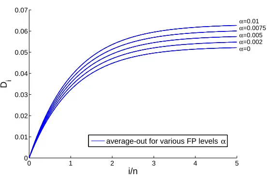
From the previous theorem, we can see that for small false positive rates α≈0, which are common in many applications, for example, intrusion detection (see Section 8 for an extensive empirical analysis), the bound approximately equals the one of the previous section; that is, we haveE(Di)≤1−νν+δwhereδ>0 is a small constant withδ→0. Inverting the bound we obtain
the useful formula
ν≥ E(Di)
1+E(Di)
, (18)
0 1 2 3 4 5 0
0.01 0.02 0.03 0.04 0.05 0.06 0.07
i/n
D i
average-out for various FP levels α
α=0.01
α=0.0075
α=0
α=0.005
α=0.002
Figure 7: Theoretical behavior of the displacement of a centroid under a poisoning attack for dif-ferent levels of false positive protectionα. The predicted displacement curve forα=0 coincides with the one shown in Figure 6.
7. Generalization to Kernels
For simplicity, we have assumed in the previous sections that the dataxi∈Rd lies in an Euclidean
space. This assumption does not add any limitations, as all our results can be generalized to the so-calledkernel functions(Sch¨olkopf and Smola, 2002). This is remarkable, as nonlinear kernels allow one to obtain complex decision functions from the simple centroid model (cf. Figure 1).
Definition 15 (Def. 2.8 in Shawe-Taylor and Cristianini, 2004) A function k:Rd×Rd → R is
called a kernel if and only if there exists a Hilbert space(
H
,h·i) and a mapφ:Rd →H
suchthat for allx,y∈Rd it holds k(x,y) =hφ(x),φ(y)i. Given a samplex1, . . . ,xn, the matrix K with
i j-th entry k(xi,xj)is calledkernel matrix.
Examination of the theoretical results and proofs of the proceeding sections reveals that they, at no point, require special properties of Euclidean spaces. Instead, all calculations can be carried out in terms of arbitrary kernels. To this end, we only need to substitute all occurrences ofx∈Rd in the
proofs by feature vectorsφ(x)∈
H
. Likewise, all occurrences of inner productshx,yi generalize to scalar productshφ(x),φ(y)iin the kernel Hilbert space. The scalar product also induces a norm, defined bykwk:=phw,wifor allw∈H
. The expectation operatorE:H
7→H
is well-defined as long asEkxkis finite, which will always be assumed (as a matter of fact, we assume thatkxkis bounded almost surely; cf. Axiom 6 and Axiom 10).is fulfilled by distributions that are symmetric with respect toc0in feature space, and thus naturally fulfilled by Gaussian distributions with meanc0(usingφ=id) or truncated Gaussians. When using kernels the symmetry assumption can be invalid, for example, for RBF kernels. However, our empirical analysis (see next section) shows that our bounds are, nevertheless, sharp in practice.
It is also worth noting that the use of kernels can impose geometric constraints on the optimal attack. Note that, in practice, the attacker can only construct attack points in the input space and not directly in the feature space. The attack is then embedded into the feature space. Thus, strictly speaking, we would need to restrict the search space to feature vectors that have a valid pre-image when using kernels. However, this can be a hard problem to solve in general (Fogla and Lee, 2006). In Proposition 11, we do not take this additional complication into account. Therefore, we overestimate the attacker. This is admissible for security analysis; it is theunderestimation of the attack capability that would have been problematic.
8. Case Study: Application to Intrusion Detection
In this section we present an experimental evaluation of the developed analytical instruments in the context of a particular computer security application: intrusion detection. After a short presentation of the application, data collection, preprocessing and model selection, we report on experiments aimed at the verification of the theoretically obtained growth rates for the attack progress as well as the computation of constant factors for specific real-life exploits.5
8.1 Anomaly-Based Intrusion Detection
Computer systems linked to the Internet are exposed to a plethora of network attacks and mali-cious code. Numerous threats, which range from simple “drive-by-downloads” of malimali-cious code to sophisticated self-proliferating worms, target network hosts every day; networked systems are generally at risk to be remotely compromised and abused for illegal purposes. Sometimes it suffices for malware to send a single HTTP-request to a vulnerable webserver to infect a vast majority of computers within minutes (e.g., the Nimda worm). While early attacks were developed rather for fun than for profit, proliferation of current network attacks is now driven by a criminal underground economy. Compromised systems are often abused for monetary gains including the distribution of spam messages and theft of confidential data. The success of these illegal businesses poses a severe threat to the security of network infrastructures. Alarming reports on an expanding dissem-ination of advanced attacks render sophisticated security systems indispensable (e.g., Microsoft, 2008; Symantec, 2008).
Conventional defenses against such malicious software rest on abuse detection; that is, iden-tifying attacks using known patterns of abuse, so-called attack signatures. While abuse detection effectively protects from known threats, it increasingly fails to be able to cope with the amount and diversity of attacks. The time span required for crafting a signature from a newly discovered attack is insufficient for protecting against rapidly propagating malicious code (e.g., Moore et al., 2002; Shannon and Moore, 2004). Moreover, recent attacks frequently use polymorphic modifications, which strongly impedes the creation of accurate signatures (Song et al., 2007). Consequently, there
is currently a strong demand for alternative techniques for detection of attacks during the course of their propagation.
Anomaly detection methods provide a means for identifying unknown and novel attacks in network traffic and thereby complement regular security defenses. The centroid anomaly detection is especially appealing because of its low computational complexity.6 It has been successfully used in several well-known intrusion detection systems (e.g., Hofmeyr et al., 1998; Lazarevic et al., 2003; Wang and Stolfo, 2004; Laskov et al., 2004b; Wang et al., 2005, 2006; Rieck and Laskov, 2007).
8.2 Data Corpus and Preprocessing
The data to be used in our case study was collected by recording real HTTP traffic for 10 days at Fraunhofer Institute FIRST. We consider the data at the level of HTTP requests which are the basic syntactic elements of the HTTP protocol. To transform the raw data into HTTP requests, we remove packet headers from the Ethernet, IP and TCP layers, and merge requests spread across multiple packets. After this point, we consider only request bodies (viewed as a byte string) to be our data point. The resulting data set comprises 145,069 requests of the average length of 489 bytes, from which we randomly drew a representative subset of 2950 data points. This data is referred to as the normal data pool.
The malicious data pool is obtained by a similar procedure applied to the network traffic gen-erated by examples of real attacks used for penetration testing.7 It contains 69 attack instances from 20 real exploits obtained from the Metasploit penetration testing framework.8 Attacks were launched in a virtual network and normalized to match the characteristics of the innocuous HTTP requests (e.g., URLs were changed to that of a real web server).
As byte sequences are not directly suitable for the application of machine learning algorithms, we deploy ak-gram spectrum kernel (Leslie et al., 2002; Shawe-Taylor and Cristianini, 2004) for the computation of inner products. This kernel represents a linear product in a feature space in which dimensions correspond to subsequences of lengthkcontained in input sequences. To enable fast comparison of large byte sequences (a typical sequence length is 500–1000 bytes), efficient algorithms using sorted arrays (Rieck and Laskov, 2008) were implemented. Furthermore, kernel values are normalized according to
k(x,x¯)7−→ p k(x,x¯)
k(x,x)k(x¯,x¯) (19)
to avoid a dependence on the length of a request payload. The resulting inner products were sub-sequently used by an RBF kernel. Notice that if k is a kernel (in our case it is; see Leslie et al., 2002), then the kernel normalized by Equation (19) is a kernel, too. For example, this can be seen by noting that, for any kernel matrix, this normalization preserves its positive definiteness as it is a columnwise operation and thus can only change the principal minors by a constant factor.
8.3 Learning Model
The feature space selected for our experiments depends on two parameters: thek-gram length and the RBF kernel width σ. Prior to the main experiments aimed at the validation of the proposed
security analysis techniques, we investigate optimal model parameters in our feature space. The parameter range considered isk=1,2,3 and σ=2−5,2−4.5, ...,25. Each of the 69 attack instances is represented by a feature vector. We refer to these embedded attacks as theattack points; that is, the points in the feature space that the adversary would like to have declared as non-anomalous.
To carry out model selection, we randomly partitioned the innocuous corpus into disjoint train-ing, validation and test sets (of sizes 1000, 500 and 500). The training set is used for computing the centroid, the validation set is used for model selection, and the test set is used to evaluate the detec-tion performance of the centroid. The training set is comprised of the innocuous data only, as the online centroid learner assumes clean training data. The validation and test sets are mixed with 10 randomly chosen attack instances. We thereby ensure that none of the attack instances mixed into the validation set has a class label that also occurs in the test data set. When sampling, we realize this requirement by simply skipping instances that would violate this condition.9For each partition, an online centroid learner model is trained on a training set and evaluated on a validation and a test set, using the normalized AUC[0,0.01] (area under the ROC-curve for false positive rates less that 0.01) as a performance measure.10 For statistical significance, model selection is repeated 1000 times with different randomly drawn partitions. The average values of the normalized AUC[0,0.01] for the differentkvalues on test partitions are given in Table 2.
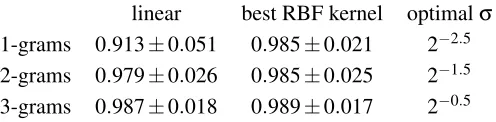
It can be seen that the 3-gram model consistently shows better AUC values for both the linear and the best RBF kernels. We have chosen the linear kernel for the remaining experiments since it allows one to carry out computations directly in the input space with only a marginal penalty in detection accuracy.
linear best RBF kernel optimalσ
1-grams 0.913±0.051 0.985±0.021 2−2.5 2-grams 0.979±0.026 0.985±0.025 2−1.5 3-grams 0.987±0.018 0.989±0.017 2−0.5
Table 2: AUC for the linear kernel, the best RBF kernel and the optimal bandwidthσ.
8.4 Intrinsic HTTP Data Dimensionality
As it was shown in Sec. 4.2.3, the dimensionality of the training data plays a crucial role in the (in)security of the online centroid learner when using the nearest-out update rule. In contrast, the displacement under the average-out rule is independent of the input dimensionality; we therefore focus on the nearest-out rule in this section. For the intrusion detection application at hand, the dimensionality of the chosen feature space (k-grams withk=3) is 2563, that is, it is rather high. One would thus expect a dramatic impact of the dimensionality on the displacement (an thus the insecurity) of the learner. However, the real progress rate depends on theintrinsicdimensionality of the data. When the latter is smaller than the size of the training data, an attacker can compute a PCA of the data matrix (Sch¨olkopf et al., 1998) and project the original data into the subspace spanned by a smaller number of informative components. The following theorem shows that the dimensionality of the relevant subspace in which attack takes place is bounded by the size of the
training datan, which can be much smaller than the input dimensionality, typically in the range of 100–1000 for realistic applications.
Theorem 16 There exists an optimal solution of problem (11) satisfying
x∗i ∈ span(a,x1, ...,xn).
The above theorem, which also can be used as a representer theorem for “kernelization” of the optimal greedy attack, shows that the attack’s efficiency cannot be increased beyond dimensions withd≥n+1. The proof is given in Appendix A.1.
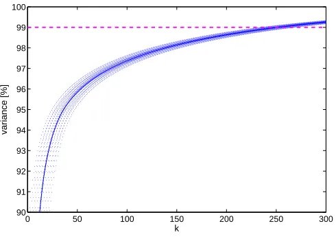
To determine the intrinsic dimensionality of possible training sets drawn from HTTP traffic, we randomly draw 1000 elements from the innocuous pool, calculate a linear kernel matrix in the space of 3-grams and compute its eigenvalue decomposition. We then determine the number of leading eigen-components as a function of the percentage of variance preserved. The results averaged over 100 repetitions are shown in Figure 8.
0 50 100 150 200 250 300
90 91 92 93 94 95 96 97 98 99 100
k
variance [%]
Figure 8: Intrinsic dimensionality of the embedded HTTP data. The preserved variance is plotted as a function of the number of eigencomponents,k, employed for calculation of variance (solid blue line). The tube indicates standard deviations.
It can be seen that 250 kernel PCA components are needed to preserve 99% of the variance. This implies that, although the effective dimensionality of the HTTP traffic is significantly smaller than the number of training data points, it still remains sufficiently high so that the attack progress rate approaches 1, which is similar to the simple average-out learner.
8.5 Geometrical Constraints of HTTP Data