Adaptive Exact Inference in Graphical Models
¨
Ozg ¨ur S ¨umer [email protected]
Department of Computer Science University of Chicago
1100 E. 58th Street Chicago, IL 60637, USA
Umut A. Acar [email protected]
Max-Planck Institute for Software Systems MPI-SWS Campus E 1 4
D-66123 Saarbruecken, Germany
Alexander T. Ihler [email protected]
Donald Bren School of Information and Computer Science University of California, Irvine
Irvine, CA 92697 USA
Ramgopal R. Mettu [email protected]
Electrical and Computer Engineering Department University of Massachusetts, Amherst
151 Holdsworth Way Amherst, MA 01003, USA
Editor: Neil Lawrence
Abstract
Many algorithms and applications involve repeatedly solving variations of the same inference prob-lem, for example to introduce new evidence to the model or to change conditional dependencies. As the model is updated, the goal of adaptive inference is to take advantage of previously com-puted quantities to perform inference more rapidly than from scratch. In this paper, we present algorithms for adaptive exact inference on general graphs that can be used to efficiently compute marginals and update MAP configurations under arbitrary changes to the input factor graph and its associated elimination tree. After a linear time preprocessing step, our approach enables updates to the model and the computation of any marginal in time that is logarithmic in the size of the input model. Moreover, in contrast to max-product our approach can also be used to update MAP config-urations in time that is roughly proportional to the number of updated entries, rather than the size of the input model. To evaluate the practical effectiveness of our algorithms, we implement and test them using synthetic data as well as for two real-world computational biology applications. Our experiments show that adaptive inference can achieve substantial speedups over performing complete inference as the model undergoes small changes over time.
1. Introduction
Graphical models provide a rich framework for describing structure within a probability distribution, and have proven to be useful in numerous application areas such as computational biology, statistical physics, and computer vision. Considerable efforts have been made to understand and minimize the computational complexity of inferring the marginal probabilities or most likely state of a graphical model. However, in many applications we may need to perform repeated computations over a collection of very similar models. For example, hidden Markov models are commonly used for sequence analysis of DNA, RNA and proteins, while protein structure requires the definition of a factor graph defined by the three-dimensional topology of the protein of interest. For both of these types of models, it is often desirable to study the effects of mutation on functional or structural properties of the gene or protein. In this setting, each putative mutation gives rise to a new problem that is nearly identical to the previously solved problem.
The changes described in the examples above can, of course, be handled by incorporating them into the model and then performing inference from scratch. However, in general we may wish to assess thousands of potential changes to the model—for example, the number of possible mutations in a protein structure grows exponentially with the number of considered sites—and minimize the total amount of work required. Adaptive inference refers to the problem of handling changes to the model (e.g., to model parameters and even dependency structure) more efficiently than performing inference from scratch. Performing inference in an adaptive manner requires a new algorithmic approach, since it requires us to balance the computational cost of the inference procedure with the reusability of its calculations. As a simple example, suppose that we wish to compute the marginal distribution of a leaf node in a Markov chain with n variables. Using the standard sum-product algorithm, upon a change to the conditional probability distribution at one end of the chain, we must performΩ(n)computation to compute the marginal distribution of the node at the other end of the chain. In such a setting, it is worth using additional preprocessing time to restructure the underlying model in such a way that changes to the model can be handled in time that is logarithmic, rather than linear, in the size of the model.
1.1 Related Work
There are numerous machine learning and artificial intelligence problems, such as path planning problems in robotics, where new information or observations require changing a previously com-puted solution. As an example, problems solved by heuristic search techniques have benefited greatly from incremental algorithms (Koenig et al., 2004), in which solutions can be efficiently up-dated by reusing previously searched parts of the solution space. The problem of performing adap-tive inference in graphical models was first considered by Delcher et al. (1995). In their work, they introduced a logarithmic time method for updating marginals under changes to observed variables in the model. Their algorithm relies on the input model being tree-structured, and can only handle changes to observations in the input model. At a high level their approach is similar to our own, in that they also use a linear time preprocessing step to transform the input tree-structured model into a balanced tree representation. However, their algorithm addresses only updates to “observations” in the model, and cannot update dependencies in the input model. Additionally, while their algorithm can be applied to general graphs by performing a tree decomposition, it is not clear whether the tree decomposition itself can be easily updated, as is necessary to remain efficient when modifying the input model. Adaptive exact inference using graph-cut techniques has also been studied by Kohli and Torr (2007). Although the running time of their method does not depend on the tree-width of the input model, it is restricted to pairwise models with binary variables or with submodular pairwise factors. Adaptivity for approximate inference has also been studied by Komodakis et al. (2008); in this work, adaptivity is achieved by performing “warm starts”. That is, a change to model is simply made at the final iteration of approximate inference and the algorithm is restarted from this state and allowed to continue until convergence.
The preprocessing technique used by Delcher et al. (1995) is inspired by a method known as
parallel tree contraction, devised by Miller and Reif (1985) to evaluate expressions on parallel
ar-chitectures. In parallel tree contraction we must evaluate a given expression tree, where internal nodes are arithmetic operations and leaves are input values. The parallel algorithm of Miller and Reif (1985) works by “contracting” both leaves and internal nodes of the tree in rounds. At each round, the nodes to eliminate are chosen in a random fashion and it can be shown that, in expec-tation, a constant fraction of the nodes are eliminated in each round. By performing contractions in parallel, the expression tree can be evaluated in logarithmic time and linear total work. Paral-lel tree contraction can be applied to any semi-ring, including sum-product (marginalization) and max-product (maximization) operators, making it directly applicable to inference problems, and it has also been used to develop efficient parallel implementations of inference (Pennock, 1998; Namasivayam et al., 2006; Xia and Prasanna, 2008).
1.2 Contributions
In this paper, we present a new framework for adaptive exact inference, building upon the work of Delcher et al. (1995). Given a factor graph G with n nodes, and domain size d (each variable can take
d different values), we require the user to specify an elimination tree T on factors. Our framework
for adaptive inference requires a preprocessing step in which we build a balanced representation of the input elimination tree in O(d3wn)time where w is the width of the input elimination tree T . We
show that this balanced representation, which we call a cluster tree, is essentially equivalent to a tree decomposition. For marginal computations, a change to the model can be processed in O(d3w·log n)
time, and the marginal for particular variable can be computed in O(d2w·log n)time. For a change
to the model that inducesℓ changes to a MAP configuration, our approach can update the MAP configuration in O(d3wlog n+dwℓlog(n/ℓ))time, without knowingℓor the changed entries in the configuration.
As in standard approaches for exact inference in general graphs, our algorithm has an expo-nential dependence on the tree-width of the input model. The dependence in our case, however is stronger: if the input elimination tree has width w, our balanced representation is guaranteed to have width at most 3w. As a result the running time of our algorithms for building the cluster tree as well as the updates have a O(d3w)multiplicative factor; updates to the model and queries however
require logarithmic, rather than linear, time in the size of the graph. Our approach is therefore most suitable for settings in which a single build operation is followed by a large number of updates and queries.
Since d and w can often be bounded by reasonably small constant factors, we know that there exists some n beyond which we would achieve speedups, but where exactly the speedups materialize is important in practice. To evaluate the practical effectiveness of our approach, we implement the proposed algorithms and present an experimental evaluation by considering both synthetic data (Section 6.1) and real data (Sections 6.2 and 6.3). Our experiments using synthetically generated factor graphs show that even for modestly-sized graphs (10−1000 nodes) our algorithm provides orders of magnitude speedup over computation from scratch for computing both marginals and MAP configurations. Thus, the overhead observed in practice is negligible compared to the speedup possible using our framework. Given that the asymptotic difference between linear and logarithmic run-times can be large, it is not surprising that our approach yields speedups for large models. The reason for the observed speedups in the smaller graphs is due to the fact that constant factors hidden by the asymptotic bounds associated with the exponential bounds are small (because they involve fast floating point operations) and because our worst-case bounds are often not attained for relatively small graphs (Section 6.1.5).
(Canutescu et al., 2003), our algorithm is nearly 7 times faster than computing minimum-energy conformations from scratch.
Several elements of this work have appeared previously in conference versions (Acar et al., 2007, 2008, 2009b). In this paper we unify these into a single framework and improve our al-gorithms and our bounds in several ways. Specifically, we present deterministic versions of the algorithms, including a key update algorithm and its proof of correctness; we derive upper bounds in terms of the tree-width, the size of the model, and the domain size; and we give a detailed exper-imental analysis.
1.3 Outline
The remainder of the paper is organized as follows. In Section 2, we give the definitions and notation used throughout this paper, along with some background on the factor elimination algorithm and tree decompositions. In Section 3, we describe our algorithm and the cluster tree data structure and how they can be used for marginalization. Then, in Section 4, we describe how updates to the underlying model can be performed efficiently. In Section 5, we extend our algorithm to compute and maintain MAP configurations under model changes. In Section 6, we show experimental results for our approach on three synthetic benchmarks and two applications in computational biology. We conclude with a discussion of future directions in Section 7.
2. Background
Factor graphs (Kschischang et al., 2001) describe the factorization structure of the function g(X)
using a bipartite graph consisting of variable nodes and factor nodes. Specifically, suppose such a graph G= (X,F)consists of variable nodes X={x1, . . . ,xn}and factor nodes F={f1, . . . ,fm}(see Figure 1a). We denote the adjacency relationship in graph G by∼G, and let Xfj=
xi∈X : xi∼Gfj be the set of variables adjacent to factor fj. For example, in Figure 1a, Xf5 ={x,v}. G is said to be consistent with a function g(·)if and only if
g(x1, . . . ,xn) =
∏
jfj
for some functions fjwhose arguments are the variable sets Xfj. We omit the arguments Xfj of each
factor fj from our formulas. In a common abuse of notation, we use the same symbol to denote a variable (resp., factor) node and its associated variable xi (resp., factor fj). We assume that each variable xitakes on a finite set of values.
In this paper we first study the problem of marginalization of the function g(X). Specifically, for any xiwe are interested in computing the marginal function
gi(xi) =
∑
X\xig(X).
Once we establish the basic results for performing adaptive inference, we will also show how our methods can be applied to another commonly studied inference problem, that of finding the config-uration of the variables that maximizes g, that is,
X∗=arg max X g(X).
f3
f4
f5 f6
f2
f1
z
y
x v
w
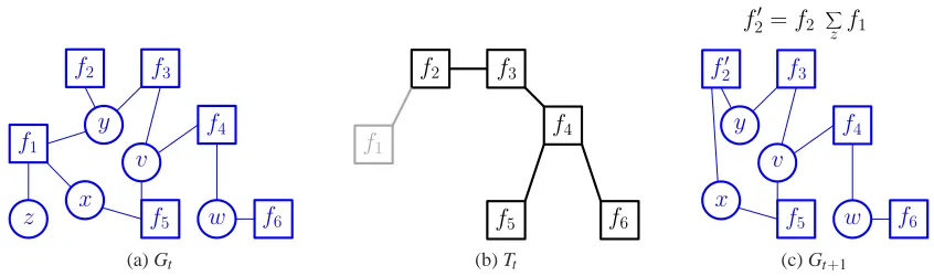
(a) Gt
f3
f4
f5 f6
f2
f1
(b) Tt
f3
f4
f5 f6
y
x v
w f2′
f2′ =f2
X z f1
(c) Gt+1
Figure 1: Factor elimination. Factor elimination takes a factor graph G1 and an elimination tree T1 as input and sequentially eliminates the leaf factors in the elimination tree. As an
example, to eliminate f1 in iteration t, we first marginalize out any variables that are
only adjacent to the eliminated factor, and then propagate this information to the unique neighbor in Tt, that is, f2′= f2∑zf1.
2.1 Factor Elimination
There are various essentially equivalent algorithms proposed for solving marginalization problems, including belief propagation (Pearl, 1988) or sum-product (Kschischang et al., 2001) for tree-structured graphs, or more generally bucket elimination (Dechter, 1998), recursive conditioning (Darwiche and Hopkins, 2001), junction-trees (Lauritzen and Spiegelhalter, 1988) and factor elimi-nation (Darwiche, 2009). The basic structure of these algorithms is iterative; in each iteration partial marginalizations are computed by eliminating variables and factors from the graph. The set of vari-ables and factors that are eliminated at each iteration is typically guided by some sort of auxiliary structure on either variables or factors. For example, the sum-product algorithm simply eliminates variables starting at leaves of the input factor graph. In contrast, factor elimination uses an
elimina-tion tree T on the factors and eliminates factors starting at leaves of T ; an example eliminaelimina-tion tree
is shown in Figure 1b.
For a particular factor fj, the basic operation of factor elimination eliminates fj in the given model and then propagates information associated with fjto neighboring factors. At iteration t, we pick a leaf factor fj in Tt and eliminate it from the elimination tree forming Tt+1. We also remove fjalong with all the variables
V
j⊆X that appear only in factor fj from Gt forming Gt+1. Let fk befj’s unique neighbor in Tt. We then partially marginalize fj, and update the value of fk in Gt+1and Tt+1with
λj=
∑
Vj
fj, fk′=fkλj.
For reasons that will be explained in Section 3.1, we use the notationλi to represent the partially marginalized functions; for standard factor elimination these operations are typically combined into a single update to fk. Finally, since multiplying byλjmay make fk′ depend on additional variables, we expand the argument set of fk′ by making the arguments ofλj adjacent to fk′ in Gt+1, that is, Xf′
k:=Xfk∪Xfj\
V
j. Figure 1 gives an example where we apply factor elimination to a leaf factor f1z
y
x
v
w
f
3f
4f
5f
6f
2f
1vwx
xyz
yx yvx
xv w
ψ1={f1}
ψ2={f2} ψ3={f3}
ψ4={f4}
ψ5 ={f5} ψ6={f6}
µχ1→χ2 =λ1
µχ2→χ3 =λ2
µχ5→χ4 =λ5
µχ6→χ4 =λ6
µχ4→χ3 =λ4
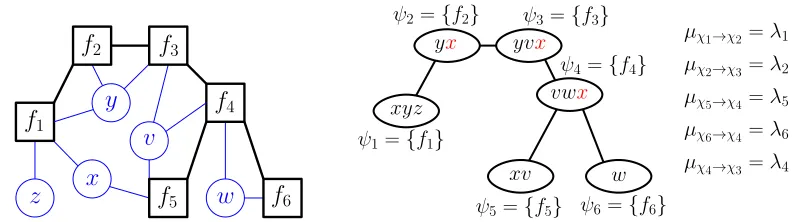
Figure 2: Factor trees and tree decompositions. A tree-decomposition (right) that is equivalent to a given elimination tree (left) can be obtained by first replacing each factor with a hyper-node that contains the variables adjacent to that factor hyper-node and then adding variables to the hyper-nodes so that the running intersection property is satisfied.
and update f1’s neighbor f2 in the elimination tree with f2′ = f2∑V1 f1. Finally, we add an edge between the remaining variables Xf1\
V
1={x}and the updated factor f′
2.
Suppose we wish to compute a particular marginal gi(xi). We root the elimination tree at a factor
fjsuch that xi∼Gfj, then eliminate leaves of the elimination tree one at a time, until only one factor remains. By definition the remaining factor fj′ corresponds to fj multiplied by the results of the elimination steps. Then, we have that gi(xi) =∑X\xi f
′
j. All of the marginals in the factor graph can be efficiently computed by re-rooting the tree and reusing the values propagated during the previous eliminations.
Factor elimination is equivalent to bucket (or variable) elimination (Kask et al., 2005; Darwiche, 2009) in the sense that we can identify a correspondence between the computations performed in each algorithm. In particular, the factor elimination algorithm marginalizes out a variable xi when there is no factor left in the factor graph that is adjacent to xi. Therefore, if we consider the operations from the variables’ point of view, this sequence is also a valid bucket (variable) elimination procedure. With a similar argument, one can also interpret any bucket elimination procedure as a factor elimination sequence. In all of these algorithms, while marginal calculations are guaranteed to be correct, the particular auxiliary structure or ordering determines the worst-case running time. In the following section, we analyze the performance consequences of imposing a particular elimination tree.
2.2 Viewing Elimination Trees as Tree-decompositions
Let G = (X,F) be a factor graph. A tree-decomposition for G is a triplet (χ,ψ,
D
) where χ={χ1,χ2, . . . ,χm}is a family of subsets of X and ψ={ψ1,ψ2, . . . ,ψm}is a family of subsets of F such that∪f∈ψiXf ⊆χi for all i=1,2, . . . ,m andD
is a tree whose nodes are the subsets χisatisfying the following properties:
1. Cover property: Each variable xi is contained in some subset belonging toχand each factor
fj∈F is contained in exactly one subset belonging toψ.
2. Running Intersection property: Ifχs,χt∈χboth contain a variable xi, then all nodesχuof the tree in the (unique) path betweenχsandχt contain xi as well. That is, the nodes associated with vertex xiform a connected sub-tree of
D
.Any factor elimination algorithm can be viewed in terms of a message-passing algorithm in a tree-decomposition. For a factor graph G, we can construct a tree decomposition (χ,ψ,
D
)that corresponds to an elimination tree T = (F,E)on G. First, we setψi={fi}andD
= (χ,E′)where(χi,χj)∈E′ is an edge in the tree-decomposition if and only if(fi,fj)∈E is an edge in the elim-ination tree T . We then initializeχ=
Xf1,Xf2, . . . ,Xfm and add the minimal number of variables
to each setχj so that the running intersection property is satisfied. By construction, the final triplet
(χ,ψ,
D
) satisfies all the conditions of a tree-decomposition. This procedure is illustrated in Fig-ure 2. The factor graph (light edges) and its elimination tree (bold edges) on the left is equivalent to the tree-decomposition on the right. We first initialize χj =Xfj for each j=1, . . . ,6 and addnecessary variables to setsχj to satisfy the running intersection property: x is added toχ2,χ3and χ4. Finally, we setψj=
fj for each j=1, . . . ,6.
Using a similar procedure, it is also possible to obtain an elimination tree equivalent to the messages passed on a given tree-decomposition. We define two messages for each edge(χi,χj)in the tree decomposition: the message µχi→χj fromχitoχjis the partial marginalization of the factors
on theχiside of
D
, and the message µχj→χifromχjtoχiis the partial marginalization of the factorson theχj side of
D
. The outgoing message µχi→χj fromχican be computed recursively using theincoming messages µχk→χi except for k= j, that is,
µχi→χj =
∑
χj\χifi
∏
(χk,χi)∈E′\{(χj,χi)}
µχk→χi. (1)
The factor elimination process can then be interpreted as passing messages from leaves to parents in the corresponding tree-decomposition. The partial marginalization functionλicomputed during the elimination of fiis identical to the message µχi→χj where fjis the parent of fiin the elimination
tree. This equivalence is illustrated in Figure 2 where each partial marginalization function λj is equal to a sum-product message µχj→χk for some k. This example assumes that f3is eliminated last.
For an elimination tree T , suppose that the corresponding tree decomposition is(χ,ψ,
D
). For the remainder of this paper, we will define the width of T to be the size of the largest set contained in χminus 1. Inference performed using T incurs a constant-factor overhead that is exponential in its width; for example, computing marginals using an elimination tree T of width w takes O(dw+1·n)time and space where n is the number of variables and d is the domain size.
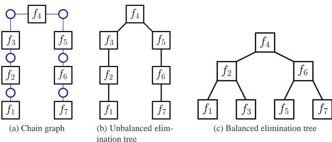
3. Computing Marginals with Deferred Factor Elimination
f3
f4
f5
f7
f6
f2
f1
(a) Chain graph
f3
f4
f5
f7
f6
f2
f1
(b) Unbalanced elim-ination tree
f
3f
4f
5f
7f
6f
2f
1(c) Balanced elimination tree
Figure 3: Balanced and unbalanced elimination trees. For the chain factor graph in (a), the elimi-nation tree in (b) has width 1 but requires O(n)steps to propagate information from leaves to the root. The balanced elimination tree in (c), for the same factor graph, has width 2 but takes only O(log n)steps to propagate information from a leaf to the root, since f3and f5
are eliminated earlier. If f1is modified, then using a balanced elimination tree, we only
need to update O(log n)elimination steps, while an unbalanced tree requires potentially
O(n)updates.
for repeated inference tasks. For example, an HMM typically used for sequence analysis yields a chain-structured factor graph as shown in Figure 3a. The obvious elimination tree for this graph is also chain-structured (Figure 3b). While this elimination tree is optimal for a single computation, suppose that we now modify the leaf factor f1. Then, recomputing the marginal for the leaf factor f7requires time that is linear in the size in the model, even though only a single factor has changed. However, if we use the balanced elimination tree shown in Figure 3c, we can compute the marginal-ization for f7in time that is logarithmic in the size of the model. While the latter elimination tree
increases the width by one (increasing the dependence on d), for fixed d and as n grows large we can achieve a significant speedup over the unbalanced ordering if we wish to make changes to the model.
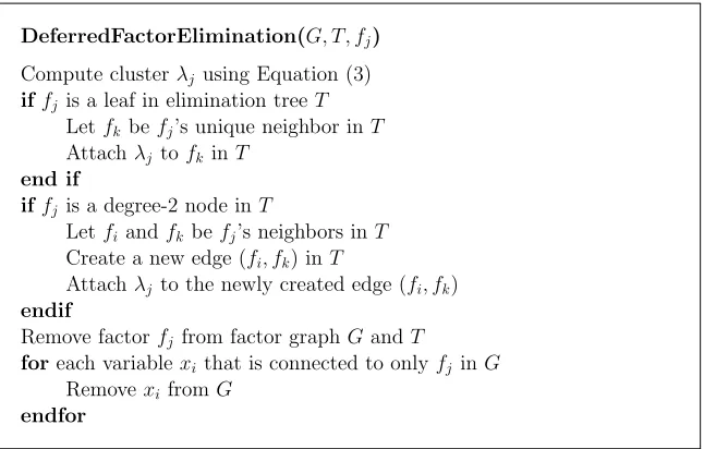
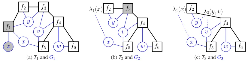
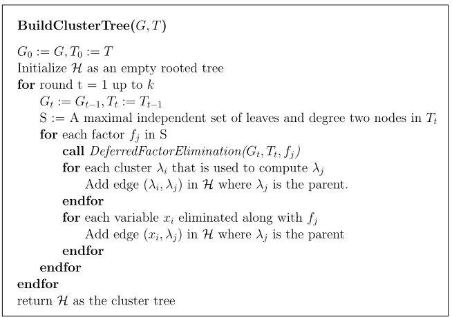
In this section we present an algorithm that generates a logarithmic-depth representation of a given elimination tree. Our primary technique, which we call deferred factor elimination, gener-alizes factor elimination so that it can be applied to non-leaf nodes in the input elimination tree. Deferred factor elimination introduces ambiguity, however, since we cannot determine the “direc-tion” that a factor should be propagated until one of its neighbors is also eliminated. We refer to the local information resulting from each deferred factor elimination as a cluster function (or, more succinctly, as a cluster), and store this information along with the balanced elimination tree. We use the resulting data structure, which we call a cluster tree, to perform marginalization and efficiently manage structural and parameter updates. Pseudocode is given in Figure 4.
DeferredFactorElimination(G, T, fj)
Compute clusterλj using Equation (3)
iffj is a leaf in elimination treeT
Letfkbefj’s unique neighbor inT
Attachλj tofkinT
end if
iffj is a degree-2 node inT
Letfiandfk befj’s neighbors inT
Create a new edge (fi, fk) inT
Attachλj to the newly created edge (fi, fk)
endif
Remove factorfj from factor graphGandT
foreach variablexithat is connected to onlyfj inG
RemovexifromG
endfor
Figure 4: Deferred factor elimination. In addition to eliminating leaves, deferred factor elimination also eliminates degree-two nodes. This operation can be simultaneously applied to an independent set of leaves and degree-two nodes.
updated. Thus, in the remainder of the paper we separate the discussion of updates applied to the input model from updates that are applied to the input elimination tree. As we will see in Section 4, the former prove to be relatively easy to deal with, while the latter require a reorganization of the cluster tree data structure.
3.1 Deferred Factor Elimination and Cluster Functions
Consider the elimination of a degree-two factor fj, with neighbors fiand fkin the given elimination tree. We can perform a partial marginalization for fjto obtainλk, but cannot yet choose whether to update fi or fk—whichever is eliminated first will needλk for its computation. To address this, we define deferred factor elimination, which removes the factor fjand saves the partial marginalization
λj as a cluster, leaving the propagation step to be decided at a later time. In this section, we show how deferred factor elimination can be performed on the elimination tree, and how the intermediate cluster information can be saved and also used to efficiently compute marginals.
For convenience, we will segregate the process of deferred factor elimination on the input model into rounds. In a particular round t (1≤t≤n), we begin with a factor graph Gt and an elimination tree Tt, and after performing some set of deferred factor eliminations, we obtain a resulting factor graph Gt+1 and elimination tree Tt+1 for the next round. For the first round, we let G1=G and T1=T . Note that since each factor is eliminated exactly once, the number of total rounds depends
on the number of the factors eliminated in each round.
f3
f4
f5 f6
f2
y
x v
w z
f1
(a) T1andG1
f4
f5 f6
f2
y
x v
w
λ1(x) f3
(b) T2andG2
f4
f5 f6
f2
y
x v
w
λ1(x) λ 3(y, v)
(c) T3andG3
Figure 5: Deferred factor elimination. (a) An elimination tree T1 (bold elges), with variable
de-pendencies shown with light edges for reference. To eliminate a leaf node f1, we sum
out variables that are not attached to any other factors (shaded), resulting in the cluster functionλ1 and new elimination tree T2 in (b). To eliminate a degree-two node f3, we
replace it withλ3attached to the edge(f2,f4), giving tree T3shown in (c).
to an edge incident to fj. In the factor graph Gt+1, we remove allλk∈
C
Tt(fj)and variablesV
j⊂Xthat do not depend on any factors other than fjorλk∈
C
Tt(fj). Finally, we replace fjwithλj, givenby
λj=
∑
Vj
fj
∏
λk∈CTt(fj)
λk. (2)
The clusterλjis referred as a root cluster if degTt(fj) =0, a degree-one cluster if degTt(fj) =1, and
a degree-two cluster if degTt(fj) =2. Figure 5 illustrates the creation of degree-one and degree-two clusters, and the associated changes to the elimination tree and factor graph. We first eliminate f1by
replacing it with degree-one clusterλ1(x) =∑zf1(x). Clusterλ1is attached to factor f2and the set
of clusters around f2is
C
T2(f2) ={λ1,λ3}. We then eliminate a degree-two factor f3by replacing it with degree-two clusterλ3(y,v) = f3(y,v). This connects f2to f4in the elimination tree, and places λ3on the newly created edge.We note that the correctness of deferred factor elimination follows from the correctness of stan-dard factor elimination. To perform marginalization for any particular variable, we can simply instantiate a series of propagations, at each step using a cluster function that has already been com-puted in one of the aforementioned rounds.
To establish the overall running time of deferred factor elimination we first explain how the clus-ters we compute can be interpreted in the tree-decomposition framework. Recall that in Section 2.2, we established an equivalence between clusters and messages in the tree-decomposition in the case where only leaf factors in the elimination tree are eliminated. We can generalize this relationship to the case where degree-two factors are also eliminated. As discussed earlier in Section 2.2, the equivalent tree-decomposition(χ,ψ,
D
) of an elimination tree T = (F,E) consists of a treeD
on hyper-nodesχ={χ1, . . . ,χm}with the same adjacency relationship with the factors{f1, . . . ,fm}inT .
A degree-one clusterλj produced after eliminating a leaf fj factor in T is a partial marginaliza-tion of the factors on a sub-tree of T . Let fk be fj’s unique neighbor in the elimination tree when it is eliminated. This impliesλj=µχt→χk for some t as previously shown in Section 2.2. Note that
A degree-two cluster λj produced after eliminating a degree-two factor fj in T is a partial marginalization of the factors in a connected subgraph S⊂T such that S and T\S are connected by
exactly two edges. Let(fi,fc)and(fd,fk)be these edges, where fcand fd belong to S and fiand
fk are outside of S (we will show how these “boundary” edges can be efficiently computed in Sec-tion 3.2). We interpretλj as an intermediary function that enables us to compute an outgoing mes-sage µχd→χk by using onlyλj and the incoming message µχj→χc, that is, µχd→χk =∑χk\χjλiµχj→χc.
These intermediate functions are in fact the mechanism that allows us avoid long sequences of mes-sage passing. For example in Figure 5,λ3 can be used to compute the message µχ3→χ4 using only µχ2→χ3, that is, µχ3→χ4(x,v) =∑yµχ2→χ3(x,y)λ3(y,v).
Finally, we note that we have a single root cluster that is just a marginalization of all of the factors in the factor graph. Using the relationships established above between cluster functions and messages in a tree decomposition, we give the running time of deferred factor elimination on a given elimination tree and input factor graph.
Lemma 1 For an elimination tree with width w, the elimination of leaf factors takesΘ(d2w)time and produces a cluster of sizeΘ(dw), where d is the domain size of the variables in the input factor
graph. The elimination of degree-two vertices takes Θ(d3w) time and produces a cluster of size
Θ(d2w).
Proof Each degree-one cluster has size O(dw)because it is equal to a sum-product message in the equivalent tree-decomposition. For a degree-two vertex fj, the clusterλj can be interpreted as an intermediary function that enables us to compute the outgoing messages µχc→χi and µχd→χk using
the incoming messages µχk→χd and µχi→χcfor someχc,χd,χiandχkwhere fiand fkare neighbors of fjin the elimination tree during its elimination. The set of variables involved in these computations is (χi∩χc)∪(χk∩χd) which is bounded by 2w. Hence, the cluster fi that computes the partial marginalization of the factors that are between(fd,fk)and(fi,fc)has size O(d2w). Moreover, these bounds are achieved ifχi∩χcandχk∩χkare disjoint and each has w variables.
We now establish the running times of calculating cluster functions, by bounding the number of variables involved in computing a cluster. We first show that when a leaf node fj is eliminated, the set of variables involved in the computation is χj∪χk where fk is fj’s neighbor. For all the degree-one clusters of fj, their argument set is a subset of χj, so the product in Equation (2) can be computed in O(dw)time. There can be a clusterλ
con the edge(fj,fk)whose argument set has to be subset ofχj∪χk. If there is such a cluster, the cost of computing the product in Equation (2) becomes O(d2w). This bound is achieved when there is a degree-two cluster and χ
j and χk are disjoint.
When a degree-two factor fj is eliminated, the set of variables involved in the computation is
χi∪χj∪χk where fi and fk are neighbors of fj. As shown above, the argument set of degree-one clusters is a subset ofχj. This cluster can have degree-two clusters on edges(fi,fj)and(fj,fk), and in this case, computation of a degree-two cluster takes O(d3w)time. This upper bound is achieved
when the setsχi,χj andχk are disjoint.
BuildClusterTree(G, T)
G0:=G, T0:=T
InitializeHas an empty rooted tree forround t = 1 up tok
Gt:=Gt−1, Tt:=Tt−1
S := A maximal independent set of leaves and degree two nodes inTt
foreach factorfj in S
callDeferredFactorElimination(Gt, Tt, fj)
foreach clusterλi that is used to computeλj
Add edge (λi, λj) inHwhereλj is the parent.
endfor
foreach variablexieliminated along withfj
Add edge (xi, λj) inHwhereλj is the parent
endfor endfor endfor
returnHas the cluster tree
Figure 6: Hierarchical clustering. Using deferred factor elimination, we can construct a balanced cluster tree data structure that can be used for subsequent marginal queries.
we can bring the complexity of computing Equation (2) down to O(dw)for each factor.
3.2 Constructing a Balanced Cluster Tree
In this section, we show how performing deferred factor elimination in rounds can be used to create a data structure we call a cluster tree. As variables and factors are eliminated through deferred factor elimination, we build the cluster tree using the dependency relationships among clusters (see Figure 6). The cluster tree can then be used to compute marginals efficiently, and as we will see, it can also be used to efficiently update the original factor graph or elimination tree.
For a factor graph G= (X,F)and an elimination tree T , a cluster tree
H
= (X∪C,E)is a rooted tree on variables and clusters X∪C where C is the set of clusters. The edges E represent thedepen-dency relationships among the quantities computed while performing deferred factor elimination. When a factor fj is eliminated, clusterλj is produced by Equation (2). All the variables
V
j and clustersC
(fj)removed in this computation becomeλj’s children. For a clusterλj, the boundary∂j is the set of edges in T that separates the collection of factors that is contracted intoλjfrom the rest of the factors.f3
f4
f5
f6
f2
f1
z
y
x
v
w
(a) Factor Graph G
z
∂3 ∂5 ∂6
∂4
∂2
∂1 ∂
4={(f2, f3)}
∂2=∅
∂1={(f1, f2)}
∂5={(f4, f5)}
∂6={(f4, f6)}
λ1
λ2
λ4
λ6
λ5
λ3
∂3={(f2, f3),(f3, f4)}
y
v x
w
(b) Cluster TreeH
Figure 7: Cluster Tree Construction. To obtain the cluster tree in (b), eliminations are performed in the factor graph G (a) in the following order: f1,f3,f5and f6in round 1, f4in round
2 and f2 in round 3. The cluster-tree (b) representing this elimination is annotated by
boundaries.
boundary ofλj can be computed by
∂j=E(fj)△∂1△∂2△. . .△∂k
where ∂i is the boundary of cluster λi and △ is the symmetric set difference operator. An ample cluster tree, along with explicitly computed boundaries, is given in Figure 7b. For ex-ample the boundary of the cluster λ4 is computed by ∂4 =E(f4)△∂3△∂5△∂6 where E(f4) =
{(f2,f4),(f4,f5),(f4,f6)}.
Theorem 2 Let G= (X,F)be a factor graph with n nodes and T be an elimination tree on G with width w. Constructing a cluster tree takesΘ(d3w·n)time.
Proof During the construction of the cluster tree, every factor is eliminated once. By Lemma 1, each such elimination takes O(d3w)time.
For our purposes it is desirable to perform deferred factor elimination so that we obtain a cluster tree with logarithmic depth. We call this process hierarchical clustering and define it as follows. We start with T1=T and at each round i we identify a set K of degree-one or -2 factors in Tiand apply deferred factor elimination to this independent set of factors to construct Ti+1. This procedure ends
once we eliminate the last factor, say fr. We makeλr the root of the cluster tree. At each round, the set K⊂F is chosen to be a maximal independent set, that is, for fi,fj ∈K, fi6∼fj in T , and no other factor fk can be added to K without violating independence. The sequence of elimination trees created during the hierarchical clustering process will prove to be useful in Section 4, when we show how to perform structural updates to the elimination tree. As an example, a factor graph
G, along with its associated elimination tree T =T1, is given in Figure 7a. In round 1, we eliminate
a maximal independent set{f1,f3,f5,f6}and obtain T2. In round 2 we eliminate f4, and finally in
round 3 we eliminate f2. This gives us the cluster tree shown in Figure 7b.
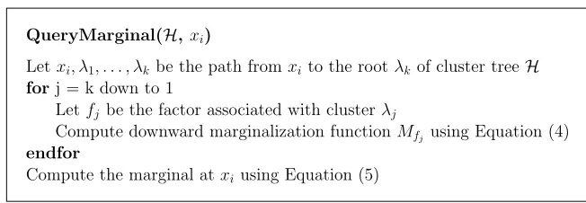
QueryMarginal(H,xi)
Letxi, λ1, . . . , λkbe the path from xito the rootλkof cluster tree H
forj = k down to 1
Letfj be the factor associated with clusterλj
Compute downward marginalization functionMfj using Equation (4)
endfor
Compute the marginal atxi using Equation (5)
Figure 8: Performing Marginalization with a Cluster Tree. Computing any particular marginal in the input factor graph corresponds to a root-to-leaf path in the cluster tree.
Lemma 3 For any factor graph G= (X,F)with n nodes and any elimination tree T , the cluster tree obtained by hierarchical clustering has depth O(log n).
Proof Let the elimination tree T = (F,E)have a leaves, b degree-two nodes and c degree-3 or more nodes, that is, m=a+b+c where m is the number of factors. Using the fact that the sum of the
degrees of the vertices is twice the number of edges, we get 2|E| ≥a+2b+3c. Since a tree with
m vertices have m−1 edges, we get 2a+b−2≥m. On the other hand, a maximal independent set
of degree-one and degree-two vertices must have size at least a−1+ (b−a)/3≥m/3, since we can eliminate at least a third of the degree-two vertices that are not adjacent to leaves. Therefore at each round, we eliminate at least a third of the vertices, which in turn guarantees that the depth of the cluster tree is O(log n).
3.3 Computing Marginals
Once a balanced cluster tree
H
has been constructed from the input factor graph and elimination tree, as in standard approaches we can compute the marginal distribution of any variable xiby prop-agating information (i.e., partial marginalizations) through the cluster tree. For any fixed variablexi, let λ1,λ2, . . . ,λk be the sequence from xi to the root λk in the cluster tree
H
. We now de-scribe how to compute the marginal for xi (see Figure 8 for pseudocode). For each factor fj, let∂j contain neighbors fa and fb of fj (i.e., neighboring factors at the time fj is eliminated). This information can be obtained easily, since fa and fb are ancestors of fj in the cluster tree, that is,
fa,fb∈
fj+1,fj+2, . . . ,fk . For convenience we state our formulas as if there are two neighbors in the boundary; in the case of degree-one clusters, terms associated with one of the neighbors, say
fb, can be ignored in the statements below. First, we compute a downward pass of marginalization functions fromλktoλ1given by
Mfj =
∑
Y\Xλj
fjMfaMfb
∏
f∈Cj\{fj−1}
f, (3)
information in the path aboveλj. Then, the marginal for variable xiis
gi(xi) =
∑
Y\{xi}Mf1
∏
f∈C1
f (4)
where Y is the set of variables that appear in the summands. Combining this approach with Lemmas 1 and 3, we have the following theorem.
Theorem 4 Consider a factor graph G with n nodes and let T be an elimination tree with width w. Then, Equation (4) holds for any variable xiand can be computed in O(d2wlog n)time.
Proof The correctness of Equation (4) follows when each marginalization function Mfj is viewed
as a sum-product message in the equivalent tree-decomposition. To prove the latter, we will show that for∂j={(fc,fa),(fd,fb)}, Mfa and Mfb are equal to the tree-decomposition messages µχa→χc
and µχb→χd, respectively. This can be proven inductively starting with Mfk. First, note that the
base case holds trivially. Then, using the inductive hypothesis, we assume that Mfa =µχa→χc and Mfb =µχb→χd. Now, there has to be a descendantλℓ ofλj such that(fe,fj)∈∂ℓ. By multiplying
with the degree-two clusters in
C
j\fj−1 , we can convert the messages µχa→χc and µχb→χd to the
messages into fj. Applying Equation (1) then gives Mfj =µχj→χe as desired.
For the running time, we observe that each message computation is essentially the same proce-dure as eliminating a leaf factor, therefore each message has size O(dw)and takes O(d2w)time to
compute by Lemma 1.
We note that it is also possible to speed-up successive marginal queries by caching the down-ward marginalization functions in Equation (3). For example, if we query all variables as described above, we compute O(n log n)many downward marginalization messages. However, by caching the downward marginalization functions in the cluster tree, we can compute all marginals in O(d2w·n)
time, which is optimal given the elimination ordering. As we will see in Section 4.1, the bal-anced nature of the cluster tree allows us to perform batch operations efficiently. In particular, for marginal computation, using the caching strategy above, any set ofℓmarginals can be computed in
O(d2wℓlog(n/ℓ))time. 4. Updates
The preceding sections described the process of constructing a balanced, cluster tree elimination ordering from a given elimination tree, and how to use the resulting cluster tree to compute marginal distributions. However, the primary advantage of a balanced ordering lies in its ability to adapt to changes and incorporate updates to the model. In this section, we describe how to efficiently update the cluster tree data structure after changes are made to the input factor graph or elimination tree.
f
3f
4f
5f
6f
2f
1z
y
x
v
w
(a)
f
3f
4f
5f
6f
2f
1z
y
x
v
w
(b)
Figure 9: Modifying the Elimination Tree. If the factor graph in (a) is modified by removing the edge(y,f1), we can reduce the width of the elimination tree (from 3 to 2) by replacing
the edge(f1,f2)by(f1,f5).
f
3f
4f
5f
6f
2f
1z
y
x
v
w
(a)
z
λ1
λ2
λ4
λ6
λ5
λ3
y
v x
w
x
(b)
Figure 10: Modifying the arguments of factors. If the factor graph in (a) is modified by removing the edge(x,f1), we update two paths in the cluster tree, as shown in (b), from both x and λ1to the root. The position in which x is eliminated is found by bottom-up traversing of
the factors adjacent to x.
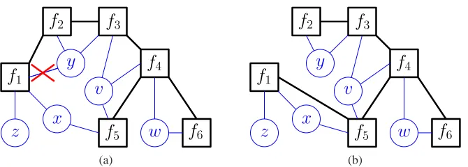
elimination tree upon changes to factors. Figure 9 illustrates such an example, in which changing a dependency in the factor graph makes it possible to reduce the width of the elimination tree.
4.1 Updating Factors With a Fixed Elimination Tree
For a fixed elimination tree, suppose that we change the parameters of a factor fj (but not its ar-guments), and consider the new cluster tree created for the resulting graph. As suggested in the discussion in Section 3, the first change in the clustering process occurs when computing λj; a change toλjchanges its parent, and so on upwards to the root. Thus, the number of affected func-tions that need to be recalculated is at most the depth of the cluster tree. Since the cluster tree is of depth O(log n)by Lemma 3, and each operation takes at most O(d3w), the total recomputation is at
most O(d3wlog n).
λ1 λ3 λ5 λ7 λ9 λ11 λ13 λ15
λ2
λ4
λ6
λ8
λ10
λ12
λ14
log(n/ℓ) log(ℓ)
Figure 11: Batch updates. After modifyingℓ=3 factors, f1,f5and f12, we update the
correspond-ing clusters and their ancestors in a bottom-up fashion. The total number of nodes visited is O(ℓlog(nℓ) +2log(ℓ)) =O(ℓlog(nℓ)).
also change. Since xi is eliminated (i.e., summed out) once every factor that depends on it has been eliminated, adding an edge may postpone elimination, while removing an edge may lead to an earlier elimination. To update the cluster tree as a result of this change, we must update all clusters affected by the change to fj, and we must also identify and update the clusters affected by earlier, or later, removal of xifrom the factor graph. In both edge addition and removal, we can update clusters fromλjto the root in O(d3wlog n)time.
We describe how to identify the new elimination point for xi in O(log n) time. Observe that the original cluster λk at which xi is eliminated is the topmost cluster in the cluster tree with the property that either fk, the associated factor, depends on xi, orλkhas two children clusters that both depend on xi. The procedure to find the new point of elimination differs for edge insertion and edge removal. First, suppose we add edge (xi,fj) to the factor graph. We must traverse upward in the cluster tree until we find the cluster satisfying the above condition. For edge removal, suppose that we remove the dependency(xi,fj). Then, xican only need to be removed earlier in the clustering process, and so we traverse downwards from the cluster where xi was originally eliminated. At any clusterλk during the traversal, if the above condition is not satisfied thenλk must have one or no children clusters that depend on xi. Ifλkhas a single child that depends on xi, we continue traversing in that direction. Ifλk has no children that depend on xi, then we continue traversing towardsλj. Note that this latter case occurs only when the paths of xi andλj to the root overlap, and thus is always possible to traverse towardλj.
Once we have identified the new cluster at which xi is eliminated, we can recalculate cluster functions upwards in O(d3wlog n)time. Therefore the total cost of performing an edge insertion or
removal O(d3wlog n). Figure 10 illustrates how the cluster tree is updated after deleting an edge in
a factor graph keeping the elimination tree fixed. After deleting(x,f1)we first update the clusters
upwards starting from λ1. Then traverse downwards to find the point at which xi is eliminated, which isλ5because f5depends on x. Finally, we updateλ5and its ancestors.
f3
f4
f5 f6
f2
f1
z y
x v
w
(a)
z λ1
λ2
λ4
λ6
λ5
λ3
y
v x
w
(b)
v w
y x
z λ1
λ2
λ3
λ4
λ5
λ6
(c)
Figure 12: Updating the elimination tree. Suppose we modify the input factor graph by removing
(y,f1)from the factor graph and replacing(f1,f2)by(f1,f5)in the elimination tree as shown in (a). The original cluster tree (b) must be changed to reflect these changes. We must revisit the decisions made during the hierarchical clustering for the affected factors (shaded).
paths must merge, and all clusters may need to be recalculated. Below level logb(ℓ), each path may be separate. Thus the total number of affected clusters isℓ+ℓlogb(n/ℓ).
Note that for edge modifications, we must also address how to find new elimination points efficiently. As stated earlier, any elimination point λk for xi satisfies the condition that it is the topmost cluster in the cluster tree with the property that either fk depends on xi, or λk has two children clusters that both depend on xi. As we update the clusters in batch, we can determine the variables for which the above condition is not satisfied until we reach the root cluster. In addition, we also mark the bottommost clusters at which the above condition is not satisfied. Starting from these marked clusters, we search downwards level-by-level until we find the new elimination points. At each step λk, we check if there is a variable xi such that xi6∼fj and only one child cluster of
λk depends on xi. If there is not, we stop the search; if there is, we continue searching towards those clusters. Since each step takes O(w)time, the total time to find all new elimination points is
O(wℓlog(n/ℓ)). We then update the clusters upwards starting from the new elimination points until the root, which takes O(d3wℓlog(n/ℓ))time.
Combining the arguments above, we have the following theorem.
Theorem 5 Let G= (X,F)be a factor graph with n nodes and
H
be the cluster tree obtained usingan elimination tree T with width w. Suppose that we makeℓchanges to the model, each consisting
of either adding or removing an edge or modifying the parameters of some factor, while holding T fixed. Then, we can recompute the cluster tree
H
′in O(d3wℓlog(n/ℓ))time.4.2 Structural Changes to the Elimination Tree
As in the previous section, we wish to recompute only those nodes in the cluster tree whose values have been affected by the update. In particular we construct the new cluster tree by stepping through the creation of the original sequence T1,T2, . . ., marking some nodes as affected if we need
to revisit the deferred elimination decision we made in constructing the cluster tree, and leaving the rest unchanged. We first describe the algorithm itself, then prove the required properties: that the original clustering remains valid outside the affected set; that after re-clustering the affected set, our clustering remains a valid maximal independent set and is thus consistent with the theorems in Section 3; and finally that the total affected set is again only of size O(log n). Since the elimination tree can be arbitrarily modified by performing edge deletions and insertions successively, for ease of exposition we first focus on how the cluster tree can be efficiently updated when a single edge in the elimination tree is inserted or deleted. For the remainder of the section, we assume that the hierarchical clustering process produced intermediate trees (T1,T2, . . . ,Tk) and that (fi,fj) is the edge being inserted or deleted.
Observe that, to update any particular round of the hierarchical clustering, for any factor fk we must be able to efficiently determine whether its associated cluster must be recomputed due to the insertion or deletion of an edge (fi,fj). A trivial way to check this would be to compute a new hierarchical clustering(T1′,T2′, . . . ,Tl′)using the changed elimination tree. Then, the clusterλk that is generated after eliminating fk depends only on the set of clusters around fk at the time of the elimination. If
C
i(fk) andC
i′(fk) are the set of clusters around fk on Ti and Ti′, respectively, then fk is affected at round i if the setsC
i(fk) andC
i′(fk) are different. Note that we considerC
i(fk) =C
i(fk) if λj ∈C
i(fk) ⇐⇒ λj ∈C
i′(fk) and the values of λj are identical in both sets. Clearly, this approach is not efficient, but motivates us to (incrementally) track whether or notC
i(fk) andC
′i(fk)are identical in a more efficient manner. To do this, we define the degree-status of the neighbors of fk, and maintain it as we update the cluster tree. Given two hierarchical clusterings
(T1= (F1,E1),T2= (F2,E2), . . . ,Tk= (Fk,/0))and(T1= (F1′,E1′),T2= (F2′,E2′), . . . ,Tl= (Fl′,/0)), we define the degree-statusσi(f)of a factor f at round i as
σi(f) = (
1 if degTi(f)≤2 or degT′
i(f)≤2 or f ∈/Fi∩F
′ i, 0 if degTi(f)≥3 and degT′
i(f)≥3.
The degree status tells us whether f is a candidate for elimination in either the previous or the new cluster tree.
At a high level, we step through the original clustering, marking factors as affected according to their degree-status. For a factor fj, ifσi(fj) =1, then fj is either eliminated or a candidate for elimination at round i in one or both of the previous and new hierarchical clusterings. Since we must recompute clusters for affected factors, if we mark fjas affected, then its unaffected neighbors should also be marked as affected in the next round. An example is shown in Figure 13. This approach conservatively tracks how affectedness “spreads” from one round to the next; we may mark factors as affected unnecessarily. However, we will be able to show that any round of the new clustering has a constant number of factors for which we must recompute clusters.
We now describe our algorithm for updating a hierarchical clustering after a change to the elimination tree. We first insert or remove the edge (fi,fj) in the original elimination tree and obtain T1′ = (V1′,E1′) where E1′ =E1∪
(fi,fj) if the edge is inserted or E1′ =E1\
(fi,fj) if deleted. For i=1,2, . . . ,l, the algorithm proceeds by computing the affected set Ai, an independent set Mi⊆Ai of affected factors of degree at most two in Ti′, and then eliminating Mi to form Ti′+1.
We let A0=
f2
f5
f3 f6 f8 f1
f4
f10 f7
f9 f12
f13 f11 f0
σ1(f3) = 0
σ1(f8) = 1 σ1(f9) = 0
(a) Round 1
f5
f3 f8
f4
f10
f9 f12
f13 f11 f1
f0
σ2(f3) = 1 σ2(f8) = 1
σ2(f9) = 0 λ2
λ6
λ9
(b) Round 2
Figure 13: Affected nodes in the clustering. By rule 2 for marking factors as affected, eliminating
f6 in the first round makesσ2(f3) =1, thereby making f1 and f5 affected. In contrast,
sinceσ2(f9) =0, f12and f13are not marked as affected. By rule 1, eliminating f7in the
first round makes f10affected.
• We obtain the new elimination tree Ti′= (Fi′,Ei′)by eliminating the factors in Mi−1from Ti−1
via deferred factor elimination subroutine.
• All affected factors left in Ti′ remain affected, namely the set Ai−1\Mi−1. We mark a
previ-ously unaffected factor f as affected if
1. f has an affected neighbor g in Ti−′ 1such that g∈Mi−1or
2. f has an affected neighbor g in Ti′such that g∈Ai−1\Mi−1withσi(g) =1.
Let Ni be the set of factors that are marked in this round according to these two rules, then
Ai= (Ai−1\Mi−1)∪Ni.
• Initialize Mi = /0 and greedily add affected factors to Mi starting with the factors that are adjacent to an unaffected factor. Let f ∈Aibe an affected factor with an unaffected neighbor
g∈Vi′\Ai. If g is being eliminated at round i we skip f , otherwise f is included in Mi if degT′
i(f)≤2. We continue traversing the set of affected factors with degree at most two and
add as many of them as we can to Mi, subject to the independence condition.
Observe that a factor f in Ti′ becomes affected either if an affected neighbor of f is eliminated at round i−1 or if f has neighbor that was affected in earlier rounds with degree-status one in Ti′. Once a factor becomes affected, it stays affected. For an unaffected factor f at round i, f ’s neighbors have to be (i) unaffected, (ii) affected with degree-status zero, or (iii) have become affected at round
i.
In order to establish that the procedure above correctly updates the hierarchical clustering, we first prove that we are able to correctly identify unaffected factors, and incrementally maintain maximal independent sets.
Lemma 6 Given T = (T1,T2, . . . ,Tk), let T′= (T1′,T2′, . . . ,Tl′)be the updated hierarchical
cluster-ing. For any round i=1. . .l, let Ti′= (Fi′,Ei′), let Pi=Fi′\Ai be the set of unaffected factors and
Ri=Pi\Fi′+1be the ones that are eliminated at round i. Then, the following statements hold:
• Ri∪Miis a maximal independent set among vertices of degree at most two in Fi′.
• For any f ∈Pi, the set of clusters around f and the set of neighbors of f are the same in Tias
Proof For the first claim, we first observe that Ri is an independent since it is contained in Mi. For maximality, assume that Ri∪Mi is not a maximal independent set among degree≤2 vertices of Fi′. Then there must be a factor f with two neighbors g,h with degrees≤2 and none of which are eliminated at round i. This triplet(f,g,h) cannot be entirely in Ai or Fi′\Ai, because the sets
Ri and Mi are maximal on their domain, namely Ri is a maximal independent set over Fi′\Ai and
Mi is a maximal independent set over Ai. On the other hand, the triplet(f,g,h)cannot be on the boundary either because the update algorithm eliminates any factor with degT′
i ≤2 if it is adjacent
to an unaffected factor that is not eliminated at round i. Therefore, Ri∪Miis a maximal independent set over degree≤2 vertices of Fi′.
We now prove the first part of the second claim by induction on i. Let
C
i(f)andC
i′(f)be the set of clusters around f in Ti and Ti′, respectively. The claim is trivially true for i=1 becauseC
i(f) =C
i′(f) =/0for all factors. Assume thatC
j(f) =C
j′(f)for all unaffected factors at round j where j=1, . . . ,i−1. Since f ∈Pi implies that f ∈Pi−1, we have thatC
i−1(f) =C
i−′ 1(f). Sincethe set of clusters around a factor changes only if any of its neighbors are eliminated, we must prove that if a neighbor of f is eliminated in Ti−1, then it must be eliminated in Ti−′ 1and vice versa;
additionally we must prove that they also generate the same clusters. Since f ∈Pi−1, the neighbors
of f in Ti′ can be unaffected, affected with degree-status zero or newly affected in round i. When an unaffected factor g is eliminated in Ti−1, it is eliminated in Ti′as well, so the resulting clusters are identical since
C
i−1(g) =C
i−′ 1(g). So any change toC
i(f) due to f ’s unaffected neighbors is replicated inC
′i(f). On the other hand, by definition we cannot eliminate a factor with degree-status zero, so they do not pose a problem even if they are affected. The last case is a newly affected neighbor g of f in Ti−1 with σi−1(g) =1. But this case is impossible because, if g is eliminated
then we would have marked f as affected in Ti via the first rule, or if g is not eliminated then by the second rule and the fact thatσi(g) =1, we would have marked f as affected in Ti. Therefore
C
i(f) =C
i′(f)for all unaffected factors. This implies that clusters of unaffected factors are identical and do not have to be recalculated in Ti′.Let
N
i(f)andN
i′(f)be the set of neighbors of f in Tiand Ti′, respectively. Proving the second part of the second claim (i.e.,N
i(f) =N
i′(f)) proceeds similarly to that forC
i(f) =C
i(f). The only difference is the initial round when i=1. In round 1, the update algorithm marks all the factors that are incident to the added or removed edges as affected, so for all unaffected factors their neighbor set must be identical in Tiand Ti′.Using this lemma, we can now prove the correctness of our method to incrementally update a hierarchical clustering.
Theorem 7 Given a valid hierarchical clustering T , let T′= (T1′,T2′, . . . ,Tl′)be the updated hierar-chical clustering, where Ti′= (F′
i,Ei′). Then, T′is a valid hierarchical clustering, that is,
• the set Mi=Fi′\Fi′+1is a maximal independent set containing vertices of degree at most two, and
• Ti′+1is obtained from Ti′by applying deferred factor elimination to the factors in Mi.
Proof Recall that Aiis the set of affected factors marked and M′i∈Aibe the independent set chosen by the algorithm. Let Pi=Fi′\Aibe the set of unaffected factors and Ri=Pi\Fi′+1be the ones that
because Mi=Ri∪Mi′. Since the update algorithm keeps the decisions made for the unaffected fac-tors, the set of eliminated vertices are precisely Mi=Ri∪Mi′ and by Lemma 6, Mi is a maximal independent set over degree-one and degree-two in Ti′. The update algorithm applies the deferred factor elimination subroutine on the set Mi′, so what remains to be shown is the saved values for Ri are the same as if we eliminate them explicitly. By Lemma 6, the factors in Ri have the same set of clusters around them in Ti and Ti′, which means that deferred factor elimination procedure will produce the same result in both elimination trees when unaffected factors are eliminated. Therefore, we can reuse the clusters in Ri.
Theorem 7 shows that our update method correctly modifies the cluster tree, and thus marginals can be correctly computed. Note that, by Lemma 3, we also have that the resulting cluster tree also has logarithmic depth. It remains to show that we can efficiently update the clustering itself. We do this by first establishing a bound on the number of affected nodes in each round.
Lemma 8 For i=1,2, . . . ,l, let Ai be the set of affected nodes computed by our algorithm after
inserting or deleting edge(fi,fj)in the elimination tree. Then,|Ai| ≤12.
Proof First, we observe that the edge (fi,fj) defines two connected components, that are either created or merged, in the elimination tree. Since an unaffected node becomes affected only if it is adjacent to an affected factor, the set of affected nodes forms a connected sub-tree throughout the elimination procedure. For the remained of the proof, we focus on the component associated with fi, and show that it has at most six affected nodes. A similar argument can be applied to the component associated with fj, thereby proving the lemma.
For round i, let Bibe the set of affected neighbors of with at least one unaffected neighbor and let Ni be the set of newly affected factors. We claim that |Bi| ≤2 and |Ni| ≤2 at every round i. This can be proven inductively: assume that |Bi|and |Ni|are at most two in round i≥0. Rule 1 for marking a factor affected can make only one newly affected factor at round i+1, in which case it is eliminated, and hence|Bi|cannot increase. Rule 2 for marking a factor affected can make two newly affected factors, as shown in the example Figure 13. What is left to be shown is that if
|Bi|=2, then rule 2 cannot create two newly affected factors and make|Bi|>2. Let Bi={fa,fb} and suppose facan force two previously unaffected factors affected in the next round. For this to happen, the degree-status of fahas to be one in round i+1. However, this cannot because famust have at least three neighbors in both Ti+1and Ti′+1. This is because it has two unaffected neighbors
plus an affected neighbor that is eventually connected to another unaffected factor through fb. Note that Figure 13 has|Bi|=1, so we can increase|Bi|by one.
We have now established the fact that the number of affected nodes can increase at most by two in each round, and it remains to be shown that the number of affected nodes is at most six in each connected component.