Nested Expectation Propagation for Gaussian Process Classification with a Multinomial Probit Likelihood

Nested Expectation Propagation for Gaussian Process Classification

with a Multinomial Probit Likelihood

Jaakko Riihim¨aki [email protected]

Pasi Jyl¨anki [email protected]

Aki Vehtari [email protected]

Department of Biomedical Engineering and Computational Science Aalto University School of Science

P.O. Box 12200 FI-00076 Aalto Finland

Editor:Neil Lawrence

Abstract

This paper considers probabilistic multinomial probit classification using Gaussian process (GP) priors. Challenges with multiclass GP classification are the integration over the non-Gaussian pos-terior distribution, and the increase of the number of unknown latent variables as the number of target classes grows. Expectation propagation (EP) has proven to be a very accurate method for approximate inference but the existing EP approaches for the multinomial probit GP classification rely on numerical quadratures, or independence assumptions between the latent values associated with different classes, to facilitate the computations. In this paper we propose a novel nested EP approach which does not require numerical quadratures, and approximates accurately all between-class posterior dependencies of the latent values, but still scales linearly in the number of between-classes. The predictive accuracy of the nested EP approach is compared to Laplace, variational Bayes, and Markov chain Monte Carlo (MCMC) approximations with various benchmark data sets. In the ex-periments nested EP was the most consistent method compared to MCMC sampling, but in terms of classification accuracy the differences between all the methods were small from a practical point of view.

Keywords: Gaussian process, multiclass classification, multinomial probit, approximate infer-ence, expectation propagation

1. Introduction

Gaussian process (GP) priors enable flexible model specification for Bayesian classification. In mul-ticlass GP classification, the posterior inference is challenging because each target class increases

the number of unknown latent variables by the number of observationsn. Typically, independent

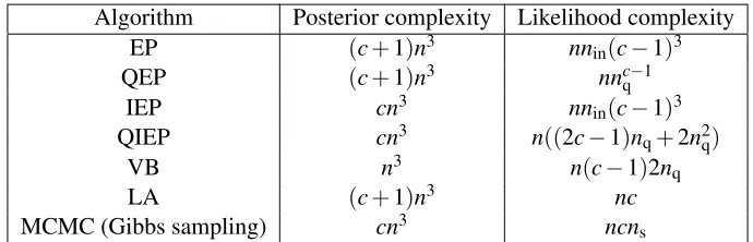
GP priors are set for the latent values for each class and this is assumed throughout this paper. Since all the latent values depend on each other through the likelihood, they become a posteriori dependent, which can rapidly lead to computationally unfavorable scaling as the number of classes

cgrows. A cubic scaling incis prohibitive, and from a practical point of view, a desired complexity

is

O

cubic scaling with respect to the number of data points is standard for full GP priors, and to reduce

As an additional challenge, the posterior inference is analytically intractable because the likelihood term related to each observation is non-Gaussian and depends on multiple latent values (one for each class).

A Markov chain Monte Carlo (MCMC) approach for multiclass GP classification with a softmax likelihood (also called a multinomial logistic likelihood) was described by Neal (1998). Sampling of the latent values with the softmax model is challenging because the dimensionality is often high and standard methods such as the Metropolis-Hastings and Hamiltonian Monte Carlo algorithms require tuning of the step size parameters. Later Girolami and Rogers (2006) proposed an alternative approach based on the multinomial probit likelihood which can be augmented with auxiliary latent variables. This enables a convenient Gibbs sampling framework in which the latent function values are conditionally independent between classes and normally distributed. If the hyperparameters

are sampled, one MCMC iteration scales as

O

for largenbecause thousands of posterior draws may be required to obtain uncorrelated posterior

samples, and strong dependency between the hyperparameters and latent values can cause slow mixing of the chains.

To speed up the inference, Williams and Barber (1998) used the Laplace approximation (LA) to approximate the non-Gaussian posterior distribution of the latent function values with a tractable Gaussian distribution. Conveniently the LA approximation with the softmax likelihood leads to an

efficient representation of the approximative posterior covariance scaling as

O

facilitates considerably the predictions and gradient-based type-II maximum a posteriori (MAP) es-timation of the covariance function hyperparameters. Later Girolami and Rogers (2006) proposed a factorized variational Bayes approximation (VB) for the augmented multinomial probit model. Assuming the latent values and the auxiliary variables a posteriori independent, a computation-ally efficient posterior approximation scheme is obtained. If the latent processes related to each

class share the same fixed hyperparameters, VB requires only one

O

iter-ation step compared to LA in whichc+1 such inverses are required in each iteration. Recently,

Chai (2012) proposed an alternative variational bounding approximation for the multinomial

lo-gistic likelihood, which results in

O

sparse approximations were determined by active inducing set selection.

Expectation propagation (EP) is the method of choice in binary GP classification where it has been found very accurate with a reasonable computational cost (Kuss and Rasmussen, 2005; Nick-isch and Rasmussen, 2008). Two types of EP approximations have been considered for the mul-ticlass setting; the first assuming the latent values from different classes a posteriori independent (IEP) and the second assuming them fully correlated (Seeger and Jordan, 2004; Seeger et al., 2006; Girolami and Zhong, 2007). Incorporating the full posterior couplings requires evaluating the

non-analytical moments ofc-dimensional tilted distributions which Girolami and Zhong (2007)

approx-imated with Laplace’s method resulting in an approximation scheme known as Laplace propagation described by Smola et al. (2004). Earlier Seeger and Jordan (2004) proposed an alternative approach where the full posterior dependencies were approximated by enforcing a similar structure for the posterior covariance as in LA using the softmax likelihood. This enables a posterior

representa-tion scaling as

O

quadrature and double-loop optimization to obtain a restricted-form site covariance approximation

for each likelihood term (Seeger and Jordan, 2004).1 _{To reduce the computational demand of EP,}

factorized posterior approximations were proposed by both Seeger et al. (2006) and Girolami and Zhong (2007). Both approaches omit the between-class posterior dependencies of the latent values

which results in a posterior representation scaling as

O

two-dimensional quadratures for evaluating the moments of the tilted distributions with the main difference being that Seeger et al. (2006) used fewer two-dimensional quadratures for computa-tional speed-up.

A different EP approach for the multiclass setting was described by Kim and Ghahramani (2006) who adopted the threshold function as an observation model. Each threshold likelihood term

fac-torizes intoc−1 terms dependent on only two latent values. This property can be used to transform

the inference onto an equivalent non-redundant model which includesn(c−1)unknown latent

val-ues with a Gaussian prior and a likelihood consisting of n(c−1) factorizing terms. It follows

that standard EP methodology for binary GP classification (Rasmussen and Williams, 2006) can be applied for posterior inference but a straightforward implementation results in a posterior

repre-sentation scaling as

O

Ghahramani (2006). Contrary to the usual EP approach of maximizing the marginal likelihood ap-proximation, Kim and Ghahramani (2006) determined the hyperparameters by maximizing a lower bound on the log marginal likelihood in a similar way as is done in the expectation maximization (EM) algorithm. Recently Hern´andez-Lobato et al. (2011) introduced a robust generalization of

the multiclass GP classifier with a threshold likelihood by incorporatingnadditional binary

indica-tor variables for modeling possible labeling errors. Efficiently scaling EP inference is obtained by making the IEP assumption.

In this paper, we focus on the multinomial probit model and describe an efficient

quadrature-free nested EP approach for multiclass GP classification that scales as

O

EP method takes into account all the posterior covariances between the latent variables, and the posterior computations scale as efficiently as in the LA approximation. We validate the proposed nested EP algorithm with several experiments. First, we compare the nested EP algorithm to various quadrature-based EP methods with respect to the approximate marginal distributions of the latent values and class probabilities with fixed hyperparameter values, and show that nested EP achieves similar accuracy in a computationally efficient manner. Using the nested EP algorithm, we study visually the utility of the full EP approximation over IEP, and compare their convergence proper-ties. Second, we compare nested EP and IEP to other Gaussian approximations (LA and VB). We visualize the accuracy of the approximate marginal distributions with respect to MCMC, illustrate the suitability of the respective marginal likelihood approximations for type-II MAP estimation of the covariance function hyperparameters, and discuss their computational complexities. Finally, we compare the predictive performance of all these methods with estimation of the hyperparameters using several real-world data sets. Since LA is known to be fast, we also test whether the predic-tive probability estimates of LA can be further improved using Laplace’s method as described by Tierney and Kadane (1986).

2. Gaussian Processes for Multiclass Classification

We consider a classification problem consisting ofd-dimensional input vectorsxi associated with

target class labelsyi∈ {1, . . . ,c}, wherec>2, fori=1, . . . ,n. All the class labels are collected in

then×1 target vectory, and all the covariate vectors are collected in the matrixX = [x1, . . . ,xn]T

of sizen×d. Given the latent function valuesfi=

locations xi, the observationsyi are assumed independently and identically distributed as defined

by the observation model p(yi|fi). The latent vectors related to all the observations are denoted by

f=

f₁1, . . . ,f_n1,f₁2, . . . ,f_n2, . . . ,f₁c, . . . ,f_ncT.

Our goal is to predict the class membership for a new input vector x∗ given the observed data

D

We set a priori independent zero-mean Gaussian process priors on the latent values related to each class, which is the usual assumption in multiclass GP classification (see, for example, Williams and Barber, 1998; Seeger and Jordan, 2004; Rasmussen and Williams, 2006; Girolami and Zhong,

2007). This specification results in the following zero-mean Gaussian prior forf:

p(f|X) =

N

whereK is acn×cnblock-diagonal covariance matrix with matricesK1,K2, . . . ,Kc (each of size

n×n) on its diagonal. Element K_ik_,j of the k’th covariance matrix defines the prior covariance

between the function values f_ik and fk_j, which is defined by the covariance function κ(xi,xj), that

is,K_ik_,j =κ(xi,xj) =Cov

h

f_ik,fk_j

i

for the latent values related to classk. A common choice for the

covariance function is the squared exponential

κse(xi,xj|θ) =σ2exp −

1 2

d

∑

k=1

l−_k2(xi,k−xj,k)2

!

,

wherexi,k is the k’th component ofxi, andθ={σ2,l1, . . . ,ld} collects the hyperparameters

gov-erning the smoothness properties of latent functions. The magnitude parameter σ2 _{controls the}

overall variance of the unknown function values, and the lengthscale parametersl1, . . . ,ld control

the smoothness of the latent function by defining how fast the correlation decreases in each input dimension. The framework allows separate covariance functions or hyperparameters for different classes but throughout this work, for simplicity, we use the squared exponential covariance function

with the sameθfor all classes.

In this paper, we consider two different observation models: the softmax model

p(yi|fi) =

exp(f_iyi)

∑c_j=1exp(f

j i)

, (1)

and the multinomial probit model

p(yi|fi) =Ep(ui)

(

c

∏

j=1,j6=yi

Φ(ui+f_iyi−f_ij) )

, (2)

where the auxiliary variableuiis distributed asp(ui) =

N

density function of the standard normal distribution. The softmax and multinomial probit models are multiclass generalizations of the logistic and the probit models respectively.

By applying Bayes’ theorem, the conditional posterior distribution of the latent values can be written as

p(f|D,θ) = 1

Zp(f|X,θ) n

∏

i=1

whereZ=p(y|X,θ) =R p(f|X,θ)∏ni=1p(yi|fi)df is known as the marginal likelihood ofθ. Both

observation models result in an analytically intractable posterior distribution and therefore approx-imate methods are needed for integration over the latent variables. Different approxapprox-imate methods are more suitable for a particular likelihood function because of the convenience of implementation: the softmax is preferable for LA because of the efficient structure and computability of the partial derivatives (Williams and Barber, 1998), while the multinomial probit is preferable for VB, EP and Gibbs sampling because of the convenient auxiliary variable representations (Girolami and Rogers, 2006; Girolami and Zhong, 2007).

3. Approximate Inference Using Expectation Propagation

In this section, we first give a general description of EP for multiclass GP classification and review some existing approaches. Then we present a novel nested EP approach for the multinomial probit model.

3.1 Expectation Propagation for Multiclass GP Classification

Expectation propagation is an iterative algorithm for approximating integrals over functions that fac-tor into simple terms (Minka, 2001b). Using EP the posterior distribution (3) can be approximated with

qEP(f|D,θ) = 1

ZEPp(f|X,θ) n

∏

i=1

˜

ti(fi|Zi˜,µ˜i,Σ˜i), (4)

where ˜ti(fi|Zi˜,µ˜i,Σ˜i) =Zi˜

N

scalar normalization terms ˜Zi, c×1 site location vectors ˜µi, andc×c site covariances ˜Σi. In the

algorithm, first the site approximations are initialized, and then each site is updated in turns. The

update for thei’th site is done by first removing the site term from the marginal posterior which

gives the cavity distribution

q−i(fi) =

N

The cavity distribution is then combined with the exact i’th likelihood term p(yi|fi) to form the

non-Gaussian tilted distribution

ˆ

p(fi) =Zˆi−1q−i(fi)p(yi|fi), (5)

which is assumed to encompass more information about the true marginal distribution. Next a

Gaussian approximation ˆq(fi) is determined for ˆp(fi) by minimizing the Kullback-Leibler (KL)

divergence KL(pˆ(fi)||qˆ(fi)), which for a Gaussian ˆq(fi)is equivalent to matching the first and second

moments of ˆq(fi)with the corresponding moments of ˆp(fi). Finally, the parameters of thei’th site

are updated so that the mean and covariance ofq(fi)are consistent with ˆq(fi). After updating the

site parameters, the posterior distribution (4) is updated. This can be done either in a sequential way,

where immediately after each site update the posterior is refreshed using a rank-c update, or in a

In binary GP classification, determining the moments of the tilted distribution requires solv-ing only one-dimensional integrals, and assumsolv-ing the probit likelihood function, these univariate integrals can be computed efficiently without numerical quadratures. In the multiclass setting, the problem is how to evaluate the multi-dimensional integrals which are required to determine the moments of the tilted distributions (5). Girolami and Zhong (2007) approximated these moments using the Laplace approximation which results in an algorithm called Laplace propagation (Smola et al., 2004). The problem with the LA approach is that the mean is replaced with the mode of the distribution and the covariance with the inverse Hessian of the log density at the mode. Because of the skewness of the tilted distribution caused by the likelihood function, the LA method can lead to inaccurate mean and covariance estimates in which case the resulting posterior approximation does not correspond to the full EP solution. Seeger and Jordan (2004) estimated the tilted moments using

multi-dimensional quadratures, but this becomes computationally demanding whencincreases, and

to achieve a posterior representation scaling linearly inc, they do an additional optimization step to

obtain a constrained site precision matrix for each likelihood term approximation.

Computations can be facilitated by using the IEP approximation where explicit between-class posterior dependencies are omitted. This simplification enables posterior computations scaling

lin-early inc. The existing approaches for the multinomial probit rely on multiple numerical

quadra-tures for each site update; the implementation of Girolami and Zhong (2007) requires a total of 2c+1 two-dimensional numerical quadratures for each likelihood term, whereas Seeger et al. (2006)

described an alternative approach where only two two-dimensional and 2c−1 one-dimensional

quadratures are needed. Later, we will demonstrate that compared to the full EP approximation, IEP underestimates the uncertainty on the latent values and in practice it may require more iterations than full EP for convergence especially if the hyperparameter setting results in strong between-class posterior couplings.

3.2 Efficiently Scaling Quadrature-Free Implementation

In this section, we present a novel nested EP approach for multinomial probit classification that does not require numerical quadratures or sampling for estimation of the tilted moments and predictive probabilities. The method also leads simultaneously to low-rank site approximations which retain all posterior couplings but results in linear computational scaling with respect to the number of

target classesc. Using the proposed nested EP approach a quadrature-free IEP approximation can

also be formed with similar computational complexity as the full EP approximation.

3.2.1 QUADRATURE-FREENESTEDEXPECTATIONPROPAGATION

Here we use the multinomial probit as the likelihood function because its product form consisting of cumulative Gaussian factors is computationally more suitable for EP than the sum of exponential

terms in the softmax likelihood. Given the meanµ−iand the covarianceΣ−i of the cavity

distribu-tion, we need to determine the normalization factor ˆZi, mean vector ˆµi, and covariance matrix ˆΣiof

the tilted distribution

ˆ

p(fi) =Zˆi−1

N

Z

N

c

∏

j=1,j6=yi

Φ(ui+f_iyi−f_ij) !

dui, (6)

which requires solving non-analytical(c+1)-dimensional integrals overfiandui. Instead of

to approximate these integrals. At first, this approach may seem computationally very demanding

since individual EP approximations are required for each of thensites. However, it turns out that

these inner EP approximations can be updated incrementally between the outer EP loops. This

scheme also leads naturally to an efficiently scaling representation for the site precisions ˜Σ−_i 1.

To form a computationally efficient EP algorithm for approximating the tilted moments, it is

helpful to consider the joint distribution offiand the auxiliary variableuiarising from (6). Defining

wi= [fTi ,ui]T and removing the marginalization over ui results in the following augmented tilted

distribution:

ˆ

p(wi) =Zˆi−1

N

∏

j=1,j6=yi

Φ(wT

i b˜i,j), (7)

whereµwi= [µT−i,0]T andΣwi is a block-diagonal matrix formed fromΣ−iand 1. Denoting the j’th

unit vector of the c-dimensional standard basis by ej, the auxiliary vectors ˜bi,j can be written as

˜

bi,j= [(eyi−ej)T,1]T. The normalization term ˆZiis the same for ˆp(fi)and ˆp(wi), and it is defined

by ˆZi=R

N

to the marginal mean and covariance of the firstccomponents ofwiwith respect to ˆp(wi).

The augmented distribution (7) is of similar functional form as the posterior distribution

result-ing from a linear binary classifier with a multivariate Gaussian prior on the weightswi and a probit

likelihood function. Therefore, the moments of (7) can be approximated with EP similarly as in linear classification (see, for example, Qi et al., 2004) or by applying the general EP formulation for latent Gaussian models described by Cseke and Heskes (2011, Appendix C). For clarity, we have summarized a computationally efficient implementation of the algorithm in Appendix A. The augmented tilted distribution (7) is approximated with

ˆ

q(wi) =Zqi−ˆ1

N

∏

j=1,j6=yi

˜

Zqiˆ,j

N

where the cumulative Gaussian functions are approximated with scaled Gaussian site functions and

the normalization constant ˆZi is approximated withZqiˆ. From now on the site parameters of ˆq(wi)

in their natural exponential form are denoted by ˜αi= [α˜i,j]Tj6=yi and ˜βi= [β˜i,j]Tj6=yi.

Note that the probit terms in Equation (7) depend on the unknown latents fi only through the

linear transformationgi=B˜Ti wi, where ˜Bi= [b˜i,j]j6=yi, that isgij=f yi i −f

j

i +ui. This relation implies

that the likelihood offi increases as the latent value associated with the correct classyi increases

compared to the latents associated with the other classes. Integration over the auxiliary variable

ui results from the conic truncation of the latent variable representation of the multinomial probit

model (see, for example, Girolami and Rogers, 2006). This relationship betweenwiandgi has two

important computational consequences. First, the fully-coupled nested EP solution can be computed

by propagating scalar moments ofg_ijwhich requires solving only one-dimensional integrals because

each probit factor in the augmented tilted distribution depends only on the scalarg_ij (see Appendix

A and references therein). Second, it can be shown that the exact mean and covariance of wi∼

ˆ

p(wi) can be solved from the respective moments of gi whose distribution is obtained by gi =

˜

BT_i wion Equation (7). Because the dimension ofgi isc−1 we can form computationally cheaper

quadrature-based estimates of the tilted moments as described in Section 3.3. We will also use the

approximate marginal moments ofgi to visualize differences in the predictive accuracy of EP and

3.2.2 EFFICIENTLYSCALING REPRESENTATION

In this section we show that the approximation (8) leads to matrix computations scaling as

O

1)n3)in the evaluation of the moments of the approximate posterior (4). The idea is to show that the

site precision matrix ˜Σ−_i 1resulting from the EP update step with ˆΣi derived from (8) has a similar

structure with the Hessian matrix of logp(yi|fi)in the Laplace approximation (Williams and Barber,

1998; Seeger and Jordan, 2004; Rasmussen and Williams, 2006).

The approximate marginal covariance offiderived from (8) is given by

ˆ

Σi=HT Σw−i1+Bi˜Ti˜B˜ T i

−1

H, (9)

where the matrix ˜Ti=diag(α˜i)is diagonal,2andHT =

Ic 0

picks up the desired components ofwi, that is,fi=HTwi. Using the matrix inversion lemma and denotingBi=HTBi˜ =eyi1T−E−yi,

whereE−yi= [ej]j6=yi and1is a(c−1)×1 vector of ones, we can write the tilted covariance as

ˆ

Σi = Σ−i−Σ−iBi(T˜i−1+11

T_+BT

i Σ−iBi)−1BTi Σ−i

= (Σ−₋1_i +Bi(T˜_i−1+11T)−1BT_i )−1. (10) Because in the moment matching step of the EP algorithm the site precision matrix is updated as

˜

Σ_i−1=Σˆ_i−1−Σ−₋1_i, we can write ˜

Σ−_i 1=Bi(T˜i−1+11 T₎−1_BT

i =Bi(T˜i−α˜i(1+1Tα˜i)−1α˜Ti )BTi . (11)

SinceBiis ac×(c−1)matrix, we see that ˜Σ−_i 1is of rankc−1 and therefore a straightforward

imple-mentation based on (11) would result into

O

a more efficient representation can be obtained by simplifying (11) further. WritingBi=−AiE−yi,

whereAi= [Ic−eyi1cT]and1cis ac×1 vector of ones, we get

˜

Σ−1

i =Ai E−yiTiE˜ −Tyi−πi(1Tcπi)−1πiT

AT_i ,

where we have definedπi=E−yiα˜i+eyi and usedBiα˜i=−Aiπi. SinceAieyi =0we can addeyieTyi

to the first term inside the brackets to obtain

˜

Σ−_i 1=AiΠiATi =Πi, where Πi=diag(πi)−(1Tcπi)−1πiπiT. (12)

The second equality can be explained as follows. MatrixΠi is of similar form with the precision

contribution of thei’th likelihood term,Wi=−∇2

filogp(yi|fi), in the Laplace algorithm (Williams

and Barber, 1998), and it has one eigenvector,1c, with zero eigenvalue: Πi1c=0. It follows that

AiΠi= (Ic−eyi1Tc)Πi=Πi−eyi0T=Πiand therefore ˜Σi−1=Πi. MatrixΠiis also precisely of the

same form as the a priori constrained site precision block that Seeger and Jordan (2004) determined by double-loop optimization of KL(qˆ(fi)||q(fi)).

In a similar fashion, we can determine a simple formula for the natural location parameter ˜

νi=Σ˜−i 1µ˜ias a function of ˜αiand ˜βi. The marginal mean offiwith respect to ˆq(wi)is given by

ˆ

µi=HiT Σ−wi1+B˜iT˜iB˜Ti

−1

Σ−_wi1µwi+B˜iβ˜i

, (13)

which we can write using the matrix inversion lemma as

ˆ

µi=ΣˆiΣ−−1iµ−i+Σ−iBi(T˜i−1+11T+BTi Σ−iBi)− 1_˜

T_i−1β˜i. (14)

Using the update formula ˜νi=Σˆ−i 1µˆi−Σ−−1iµ−i resulting from the EP moment matching step and

simplifying further with the matrix inversion lemma, the site location ˜νican be written as

˜

νi=Bi β˜i−α˜iai

=aiπi−E−yiβ˜i, (15)

where ai= (1Tβ˜i)/(1Tcπi). The site precision vector ˜νi is orthogonal with1c, that is, 1Tcν˜i =0,

which is congruent with (12). Note that with results (12) and (15), the mean and covariance of

the approximate posterior (4) can be evaluated using only ˜αi and ˜βi. It follows that the posterior

(predictive) means and covariances as well as the marginal likelihood can be evaluated with similar computational complexity as with the Laplace approximation (Williams and Barber, 1998; Ras-mussen and Williams, 2006). For clarity the main components are summarized in Appendix B. The

IEP approximation in our implementation is formed by matching thei’th marginal covariance with

diag(diag(_Σˆ_{i)), and the corresponding mean with ˆµi.}

3.2.3 EFFICIENT IMPLEMENTATION

Approximating the tilted moments using inner EP for each site may appear too slow for larger problems because typically several iterations are required to achieve convergence. However, the

number of inner-loop iterations can be reduced by storing the site parameters ˜αi and ˜βiafter each

inner EP run and continuing from the previous values in the next run. This framework where the

inner site parameters ˜αi and ˜βi are updated iteratively instead of ˜µi and ˜Σi, can be justified by

writing the posterior approximation (4) using the approximative site terms from (8):

q(f|D,θ)∝p(f|X,θ)

n

∏

i=1

Z

N

c

∏

j=1,j6=yi

˜

Zqiˆ,j

N

Calculating the Gaussian integral overui leads to the same results for ˜µi and ˜Σi as derived earlier

(Equations 12 and 15). Apart from the integration over the auxiliary variables ui, Equation (16)

resembles an EP approximation where n(c−1)probit terms of the form Φ(ui+f_iyi−f_ij) are

ap-proximated with Gaussian site functions. In accordance with the standard EP framework we form

the cavity distributionq−i(fi)by removingc−1 sites from (16) and subsequently refine ˜αi and ˜βi

using the mean and covariance of the tilted distribution (6). If we alternatively expand only thei’th

site approximation with respect touiand write the corresponding marginal approximation as

q(fi|D,θ)∝q−i(fi)

Z

N

c

∏

j=1,j6=yi

˜

Zqiˆ,j

N

we can consider updating only one of the approximative terms in (17) at a time. This is

equiva-lent to starting the inner EP iterations with the values of ˜αi and ˜βi from the previous outer-loop

The previous interpretation of the algorithm is also useful for defining damping (Minka and Laf-ferty, 2002), which is commonly used to improve the numerical stability and convergence of EP. In damping the site parameters in their natural exponential forms are updated to a convex combination

of the old and new values. Damping cannot be directly applied on the site precision matrixΠi=Σ˜−i 1

because the constrained form of the site precision (12) is lost. Instead we damp the updates on ˜αi

and ˜βi which preserves the desired structure. This can be justified with the same arguments as in

the previous paragraph where we considered updating only one of the approximative terms in (17) at a time. Convergence of the nested EP algorithm with full posterior couplings using this scheme is illustrated with different damping levels in Section 5.4.

3.3 Quadrature-Based Full EP Implementation

A challenge in forming the fully-coupled EP approximation using numerical quadratures is how to obtain a site precision structure, which results in efficiently scaling posterior computations. Seeger

and Jordan (2004) used c-dimensional Gauss-Hermite rules and determined a similar site

preci-sion matrix as in Equation (12) by optimizing KL(piˆ(fi)||q(fi)). In this section, we use the ideas

from Section 3.2 to form a simpler fully-coupled EP algorithm that uses similar approximate site

precision structures determined directly using(c−1)-dimensional quadratures instead of separate

optimizations.

We use the previously defined transformationgi=B˜Ti wi, wherewi∼pˆ(wi), and denote the tilted

mean vector and covariance matrix ofwiwith ˆµwi and ˆΣwi. Analogously, we denote the

correspond-ing moments ofgi resulting from the transformation with ˆµgi and ˆΣgi. Making the transformation

on (7) and differentiating twice with respect toµwi, it can be shown that the following relation holds

between the exact covariance matrices of the random vectorswiandgi:

ˆ

Σgi=B˜TiΣˆwiBi˜ =B˜Ti (Σ−wi1+Bi˜ΛiB˜ T

i )−1Bi˜, (18)

whereΣwi is the cavity covariance ofwi. SolvingΛifrom (18) gives

Λi=Σˆ−gi1−Σ−gi1, (19)

whereΣgi =BTi Σ−iBi+11T, and ˆΣgi can be estimated with a (c−1)-dimensional quadrature rule.

The marginal tilted covariance offi can be computed from ˆΣwi similarly as in Equations (9) and

(10), and the corresponding site precision matrix ˜Σ−_i 1can be computed as in Equation (11) withΛi

now in place of ˜Ti. This gives the following site precision structure

˜

Σ−_i 1=Bi(Λ_i−1+11T)−1BT_i ,

which depends only onΛi. The form of the site precision is similar to nested EP, except that nowΛi

is a full matrix, which would result in the unfavorable

O

we approximate Λi with its diagonal to get the same structure as in Equation (12), where now

˜

Λi=diag(diag(Λi))is used instead of ˜Ti. This results in posterior computations scaling linearly in

csimilarly as with the full nested EP approach.

To estimate the site location parameter ˜νiusing quadratures, we proceed in the same way as for

the site precision. Making the transformation on (7) and differentiating once with respect toµwi, it

can be shown that the tilted means ofwiandgiare related according to

ˆ

where ˆµwi has similar form as in Equation (13). The vectorξi corresponds to ˜βi in nested EP, and

we can solve it from (20), which results in

ξi=Σˆ−gi1µˆgi−Σ −1

gi µgi, (21)

where µgi =BT_i µ−i, and ˆµgi can be estimated using a(c−1)-dimensional quadrature. If Λi is

approximated with its diagonal, we have to substitute ˆΣ−1

gi =Λ˜i+Σ−gi1in Equation (21), which results

from the diagonal approximation ofΛi made in Equation (19). In the same way as in Equations

(13)-(15), we get the following expression for the site location

˜

νi=Bi(ξi−Λ˜i1(1+1TΛ˜i1)−11Tξi),

which depends only onξi and ˜Λi. This site location structure is similar to nested EP (15) with ξi

in place of ˜βi. Using these results, a quadrature-based full EP algorithm can be implemented in the

same way as the outer-loop of nested EP. Later in Section 5.1, we validate this approximate(c−

1)-dimensional quadrature approach by comparing the tilted moments to those of a more expensive

straightforward(c+1)-dimensional full quadrature solution.

4. Other Approximations for Bayesian Inference

In this section we discuss all the other approximations considered in this paper for multiclass GP classification. First we give a short description of the LA method. Then we show how it can be improved upon by computing corrections to the marginal predictive densities using Laplace’s method as described by Tierney and Kadane (1986). Finally, we briefly summarize the MCMC and VB approximations.

4.1 Laplace Approximation

In the Laplace approximation a second order Taylor expansion of logp(f|D,θ)is made around the

posterior mode ˆf which can be determined using Newton’s method as described by Williams and

Barber (1998) and Rasmussen and Williams (2006). This results in the posterior approximation

qLA(f|

D

N

whereW=−∇2

flogp(y|f)|f=ˆfand in whichp(y|f) =∏ni=1p(yi|fi). With the softmax likelihood (1),

the submatrix ofW related to each observation will have a similar structure withΠi in (12), which

enables efficient posterior computations that scale linearly incas already discussed in the case of

EP.

4.1.1 IMPROVINGMARGINALPOSTERIORDISTRIBUTIONS

In Gaussian process classification, the LA and EP methods can be used to efficiently form a mul-tivariate Gaussian approximation for the posterior distribution of the latent values. Recently, mo-tivated by the earlier ideas of Tierney and Kadane (1986), two methods have been proposed for improving the marginal posterior distributions in latent Gaussian models; one based on subsequent use of Laplace’s method (Rue et al., 2009), and one based on EP (Cseke and Heskes, 2011). Be-cause in classification the focus is not on the predictive distributions of the latent values but on the

numerical integration over the improved posterior approximation of the corresponding latent value f∗=f(x∗). In the multiclass setting integration over a multi-dimensional space is required which

becomes computationally demanding to perform, for example, in a grid ifcis large. To avoid this

integration, we test computing the corrections directly for the predictive class probabilities follow-ing another approach presented by Tierney and Kadane (1986). A related idea for approximatfollow-ing the predictive distribution of linear model coefficients directly with a deterministic approximation has been discussed by Snelson and Ghahramani (2005).

The posterior mean of a smooth and positive functionh(f)is given by

E[h(f)] =

R

h(f)p(y|f)p(f)d f

R

p(y|f)p(f)d f , (22)

where p(y|f) is the likelihood function and p(f) is the prior distribution. Tierney and Kadane

(1986) proposed to approximate both integrals in (22) separately with Laplace’s method. This

approach can be readily applied for approximating the posterior predictive probabilitiesp(y∗|x∗)of

class membershipsy∗∈ {1, ...,c}which are given by

p(y∗|x∗,

D

1

Z

ZZ

p(y∗|f∗)p(f∗|f,x∗,X)p(f|X)p(y|f)dfdf∗, (23)

whereZ=RRp(f∗|f,x∗,X)p(f|X)p(y|f)dfdf∗=R p(f|X)p(y|f)dfis the marginal likelihood. With a

fixed class labely∗the integrals can be approximated by a straightforward application of either LA

or EP, which is already done for the marginal likelihoodZin the standard approximations. The LA

method can be used for smooth and positive functions such as the softmax whereas EP is applicable for a wider range of models.

The integral on the right side of (23) is equivalent to the marginal likelihood resulting from a

classification problem with one additional training pointy∗. To compute the predictive probabilities

for all classes, we evaluate this extended marginal likelihood consisting ofn+1 observations with

y∗fixed to one of thecpossible class labels at a time. This is computationally demanding because

several marginal likelihood evaluations are required for each test input. Additional modifications, for example, initializing the latent values to their predictive mean implied by standard LA, could be done to speed up the computations. Since further approximations can only be expected to reduce the accuracy of the predictions, we do not consider them in this paper, and focus only on the naive implementation due to its ease of use. Since LA is known to be fast, we test the goodness of the improved predictive probability estimates using only LA, and refer to the method as LA-TKP as an extension to the naming used by Cseke and Heskes (2011).

4.2 Markov Chain Monte Carlo

Because MCMC estimates become exact in the limit of infinite sample size, we use MCMC as a gold standard for measuring the performance of the other approximations. Depending on the likelihood, we use two different sampling techniques; scaled Metropolis-Hastings sampling for the softmax function, and Gibbs sampling for the multinomial probit function.

4.2.1 SCALEDMETROPOLIS-HASTINGSSAMPLING FORSOFTMAX

p(f|D,θ)using the scaled Metropolis-Hastings sampling (Neal, 1998). Then, the hyperparameters

can be drawn from the conditional posterior p(θ|f,

D

Carlo (HMC) (Duane et al., 1987; Neal, 1996).

4.2.2 GIBBSSAMPLING FOR MULTINOMIALPROBIT

Girolami and Rogers (2006) described how to draw samples from the joint posterior using the Gibbs sampler. The multinomial probit likelihood (2) can be written in the form

p(yi|fi) =

Z

ψ(vyi_i >vk_i∀k6=yi)

c

∏

j=1

N

wherevi= [v1i, ...,vci]T is a vector of auxiliary variables, andψis the indicator function whose value

is one if the argument is true and zero otherwise. Gibbs sampling can then be employed by drawing

samples alternately for allifromp(vi|fi,yi)which is a conic truncation of the multivariate Gaussian

distribution, and from p(f|v,θ) which is a multivariate Gaussian distribution. Given v and f the

hyperparameters can be drawn, for example, using HMC.

4.3 Factorized Variational Approximation

A computationally convenient variational Bayesian approximation forp(f|

D

employing the auxiliary variable representation (24) of the multinomial probit likelihood. As shown

by Girolami and Rogers (2006), assuming f a posteriori independent ofv (which contains allvi)

leads to the following approximation

qVB(v,f|D,θ) =q(v)q(f) =

n

∏

i=1 q(vi)

c

∏

j=1 q(fj_),

where the latent values associated with the j’th class,fj_{, are independent. The posterior}

approxima-tionq(fj_{)will be a multivariate Gaussian distribution, andq(v}

i)a conic truncation of the

multivari-ate Gaussian distribution (Girolami and Rogers, 2006). Given the hyperparameters, the parameters

of q(v) and q(f) can be determined iteratively by maximizing a variational lower bound on the

marginal likelihood. Each iteration step requires determining the expectations ofviwith respect to

q(vi)which can be obtained by either one-dimensional numerical quadratures or sampling methods.

In our implementation, the hyperparametersθare determined by maximizing the variational lower

bound with fixedq(v)andq(f)similarly as in the maximization step of the EM algorithm.

5. Experiments

This section is divided into five parts. In Section 5.1 we compare nested EP to quadrature-based EP in cost and quality. In Section 5.2, we illustrate the differences of the nested EP and IEP ap-proximations in a simple synthetic classification problem. In Section 5.3, we compare visually the

quality of the approximate marginal distributions off, the marginal likelihood approximations and

5.1 Comparing Nested EP to Numerical Quadrature

In this section we first validate the accuracy of the inner EP approximation and the full quadrature method described in Section 3.3 for estimation of the tilted moments. Then we compare the accuracy and numerical cost of the nested EP approximation to several quadrature-based EP implementations. In the comparisons, we use two different types of classification data: the Glass data set from the UCI Machine Learning Repository (Frank and Asuncion, 2010), and the USPS 3 vs. 5 vs. 7 data set from the US Postal Service (USPS) database (Hull, 1994). The USPS 3 vs. 5 vs. 7 data set is defined as a three class sub-problem from the USPS repartitioned handwritten digits data by considering

classification of 3’s vs. 5’s vs. 7’s.3 _{The Glass data has six (c=6) target classes but only a small}

number of observations (n=214), whereas the USPS 3 vs. 5 vs. 7 data has only three (c=3) target

classes but a larger number of training points (n=1157). See also Table 3.

In the first experiment, we examine the tilted moments after two parallel EP outer-loop iter-ations when the parameters of the cavity distributions are clearly different from their initialized values for all site terms. We fixed the hyperparameters of the squared exponential covariance

func-tion to log(σ2_{) =1 and log(l) =1, where the small value of the magnitude parameter leads to a}

close-to-Gaussian posterior as will be discussed more in Section 5.3. The main reason for not us-ing more difficult hyperparameter values (larger magnitude) in this experiment, was that we had stability problems in the actual EP algorithm using quadratures. Stability could be improved by increasing the number of quadrature points, but this became computationally too expensive with a larger number of classes.

As a baseline approximation, we compute the normalization factors ˆZi, the mean vectors ˆµi,

and the covariance matrices ˆΣi of the tilted distribution (6) for all i=1, . . . ,n using a (c+

1)-dimensional Gauss-Hermite product rule with ten quadrature points in each dimension. We call this quadrature method QF10. This provides us a reference by which inner EP and the following

four (c−1)-dimensional Gauss-Hermite quadrature methods (see Section 3.3 for further details)

are assessed: Q5 using five and Q10 using ten quadrature points in each dimension with the full

matrixΛi, and QD5 using five and QD10 using ten quadrature points in each dimension with the

diagonal approximation ˜Λi. Note that implementing an EP algorithm using QF10, Q5 or Q10, we

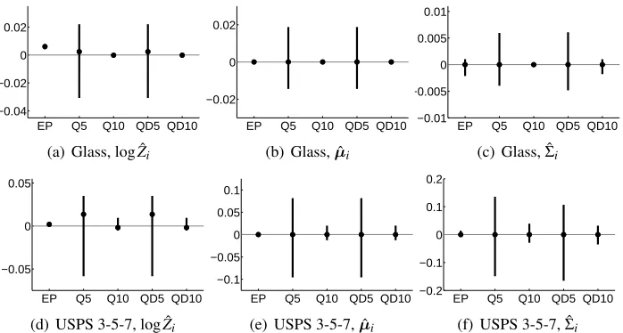
would lose the linear posterior scaling inc. Figure 1 shows the pairwise differences of log ˆZi, and

all the entries of ˆµi and ˆΣi with respect to QF10. The mean values and the 95% intervals of the

differences are illustrated. The normalization, mean and covariance are well calibrated for all the quadrature methods. Inner EP matches the mean and covariance accurately, but there is a small bias in the normalization term, probably due to the skewed tilted distributions. Variations of the

pairwise differences are small with inner EP and the(c−1)-dimensional quadratures as long as

there are enough quadrature points. Because QD10 agrees well with QF10, from now on, we use it to compute the tilted moments in the full quadrature solution, and refer to this algorithm as QEP.

In the second experiment, we compare the nested and quadrature EP algorithms in accuracy and computational cost. We use Gibbs sampling as a reference method by which nested EP and IEP, QEP, and quadrature-based IEP (QIEP) are measured. Both nested EP algorithms are implemented incrementally, so that only one inner-loop iteration per site is done at each outer-loop iteration step, which results in computational savings (see Section 3.2.3). For QIEP we use the implementation proposed by Seeger et al. (2006) with ten quadrature points for integration over the latent value from each class. We compare the absolute differences of class probabilities and latent means and

EP Q5 Q10 QD5 QD10 −0.04

−0.02 0 0.02

(a) Glass, log ˆZi

EP Q5 Q10 QD5 QD10

−0.02 0 0.02

(b) Glass, ˆµi

EP Q5 Q10 QD5 QD10

−0.01 −0.005 0 0.005 0.01

(c) Glass, ˆΣi

EP Q5 Q10 QD5 QD10

−0.05 0 0.05

(d) USPS 3-5-7, log ˆZi

EP Q5 Q10 QD5 QD10

−0.1 −0.05 0 0.05 0.1

(e) USPS 3-5-7, ˆµi

EP Q5 Q10 QD5 QD10

−0.2 −0.1 0 0.1 0.2

(f) USPS 3-5-7, ˆΣi

Figure 1: A comparison of tilted moments after two parallel EP outer-loop iterations using the

Glass and USPS 3 vs. 5 vs. 7 data sets. Using a (c+1)-dimensional Gauss-Hermite

product rule with ten quadrature points in each dimension (QF10) as a baseline result,

we compare inner EP and the following(c−1)-dimensional Gauss-Hermite quadrature

methods: five- and ten-dimensional product rules with fullΛi(Q5 and Q10) and diagonal

˜

Λi(QD5 and QD10). The mean values and the 95% intervals of the pairwise differences

of ˆZi, and all the entries of ˆµi and ˆΣi with respect to QF10 are shown. See the text for

further details.

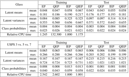
variances using the Glass and USPS 3 vs. 5 vs. 7 data sets with the same fixed hyperparameters as earlier. We split the Glass data set randomly into training and test parts, and use the predefined training and test parts for the USPS 3 vs. 5 vs. 7 data set. Table 1 reports the mean and maximum values of the element-wise differences with respect to Gibbs sampling after 30 outer-loop iterations of EP. Table 1 shows also the relative CPU times for training. From the table it can be seen that the differences in accuracy between the methods are small. For the Glass data the fully-coupled EP algorithms give slightly more accurate estimates for the mean and variances of the latents than the IEP algorithms do, but the class probabilities are in practice the same across all the methods. The main observation with the Glass data is that the CPU times of EP, IEP and QIEP are similar for

practical purposes, but QEP is clearly slower due to the unfavorable scaling inc. We acknowledge

that the performance differences in the relative CPU time are approximate and depend much on the implementation, but to reduce these effects the same outer-loop implementation was used for both nested and quadrature EP with the same fixed number of iterations. It is also worth to notice that QEP and EP have practically the same CPU times with the USPS 3 vs. 5 vs. 7 data where

the number of target classes cis only three, but both of them are slower than the IEP algorithms

due to larger n and the additional n×n inversion needed in the posterior update with the

Glass Training Test

EP QEP IEP QIEP EP QEP IEP QIEP

Latent means mean 0.048 0.047 0.058 0.067 0.043 0.043 0.055 0.058

max 0.181 0.186 0.190 0.217 0.176 0.177 0.193 0.181

Latent variances mean 0.084 0.085 0.325 0.325 0.097 0.097 0.314 0.314

max 0.553 0.560 0.656 0.667 0.571 0.572 0.643 0.655

Class probabilities mean 0.004 0.004 0.004 0.004 0.003 0.004 0.004 0.004

max 0.025 0.026 0.021 0.021 0.021 0.022 0.024 0.024

Relative CPU time 1.245 132.300 1.000 1.175

USPS 3 vs. 5 vs. 7 Training Test

EP QEP IEP QIEP EP QEP IEP QIEP

Latent means mean 0.065 0.065 0.065 0.065 0.006 0.006 0.006 0.006

max 0.266 0.288 0.266 0.266 0.203 0.202 0.199 0.199

Latent variances mean 0.167 0.167 0.167 0.167 0.215 0.215 0.216 0.215

max 0.724 0.724 0.723 0.731 1.021 1.021 1.021 1.021

Class probabilities mean 0.008 0.008 0.013 0.013 0.001 0.001 0.001 0.001

max 0.040 0.043 0.059 0.058 0.022 0.024 0.035 0.035

Relative CPU time 2.542 2.602 1.000 1.001

Table 1: A comparison of nested and quadrature-based EP in terms of accuracy and cost using the Glass and USPS 3 vs. 5 vs. 7 data sets. The table shows the element-wise mean and maximum absolute differences of the latent means and variances and the class probabilities for EP, QEP, IEP, and QIEP with respect to Gibbs sampling. See the text for further details.

small number of quadrature points (for example less than ten), from now on, we use nested EP and IEP implementations due to their stability and good computational scaling.

5.2 Illustrative Comparison of EP and IEP with Synthetic Data

In this section, we study the properties of the proposed nested EP and IEP approximations in a synthetic three-class classification problem with scalar inputs shown in Figure 2. The symbols x

(class 1), + (class 2), and o (class 3) indicate the positions of n=15 training inputs generated

from three normal distributions with means -1, 2, and 3, and standard deviations 1, 0.5, and 0.5, respectively. The left-most observations from class 1 can be better separated from the others but the observations from classes 2 and 3 overlap more in the input space. We fixed the hyperparameters of

the squared exponential covariance function at the corresponding MCMC means: log(σ2_{) =4.62}

and log(l) =0.26.

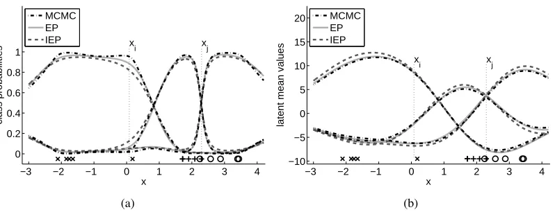
Figure 2(a) shows the predictive probabilities of all tree classes estimated with EP, IEP and

MCMC as a function of the inputx. At the class boundaries, the methods give similar predictions

−3 −2 −1 0 1 2 3 4 0

0.2 0.4 0.6 0.8 1

class probabilities

x x

i xj

MCMC EP IEP

(a)

−3 −2 −1 0 1 2 3 4

−10 −5 0 5 10 15 20

latent mean values

x x

i xj

MCMC EP IEP

(b)

Figure 2: A synthetic one-dimensional example of a three class classification problem, where the MCMC, EP and IEP approximations are compared. The symbols x (class 1), + (class 2),

and o (class 3) in the bottom of the plots indicate the positions ofn=15 observations.

Plot (a) shows the predicted class probabilities, and (b) shows the predicted latent mean

values for all three classes. The symbolsxiandxjindicate two example positions, where

the marginal distributions between the latent function values are illustrated in Figures 3 and 4. See the text for explanation.

the predictions differ, we look at the quality of the approximations made for the underlyingf. Figure

2(b) shows the approximated latent mean values which are similar at all input locations.

To illustrate the approximate posterior uncertainties off, we visualize two exemplary marginal

distributions at locations xi andxj marked in Figure 2. The MCMC samples of fi1 and fi2 (the

latents associated with classes 1 and 2 related toxi) together with a smoothed density estimate are

shown in Figure 3(a). The marginal distribution is non-Gaussian, and the latent values are more likely larger for class 1 than for class 2 indicating a larger predictive probability for class 1. The corresponding EP and IEP approximations are shown in Figures 3(b)-(c). EP captures the shape of the true marginal posterior distribution better than IEP. To illustrate the effect of these differences on the predictive probabilities, we show the unnormalized tilted distributions

ˆ

p(gi|

D

D

c

∏

k=1,k6=yi

Φ(gk_i), (25)

where the random vectorgiis defined in Section 3.2.1, andq(gi|D,xi)is the approximate marginal

obtained fromq(fi|D,xi)by a linear transformation. Note that the marginal predictive probability

for class labelyi with the multinomial probit model (2) can be obtained by appropriately forming

the transformationBiand calculating the integral overgiin (25). Figures 3(d)-(f) show the contours

of the different approximations of ˆp(gi|D,xi)fork∈ {2,3}, which for MCMC are obtained using a

smoothed estimate ofq(gi|D,xi)determined from transformed samples. The distributions are

−10 0 10 20 30 −20

−10 0 10 20

latent f i 1

latent f

i

2

MCMC

(a)

−10 0 10 20 30

−20 −10 0 10 20

latent f i 1

latent f

i

2

EP

(b)

−10 0 10 20 30

−20 −10 0 10 20

latent f i 1

latent f

i

2

IEP

(c)

0 20 40

0 20 40

g

i 2

g i

3

MCMC, p=0.95

(d)

0 20 40

0 20 40

g

i 2

gi

3

EP, p=0.88

(e)

0 20 40

0 20 40

g

i 2

g i

3

IEP, p=0.82

(f)

Figure 3: An example of a non-Gaussian marginal posterior distribution for the latent values related

to the input xi in the synthetic example shown in Figure 2. The first row shows the

distribution for the latents f_i1 and f_i2. Plot (a) shows a scatter-plot of MCMC samples

drawn from the posterior and estimated density contour levels which correspond to the areas that include approximately 95%, 90% 75%, 50%, and 25% of the probability mass. Plots (b) and (c) show the equivalent contour levels of the EP and IEP approximations (bold black lines) and the contour levels of the MCMC approximation (gray lines) for comparison. Plots (d)-(f) show contours of ˆp(gi|D,xi)forg2i andg3i. The probability for

class 1 is obtained by calculating the integral overgi, which results in approximately 0.95

for MCMC, 0.88 for EP, and 0.82 for IEP. See the text for explanation.

The second locationxj is near the class boundary, where all the methods give similar predictive

probabilities, although the latent approximations can differ notably as shown in Figures 4(a)-(c),

which visualize the marginal approximations for f2_j and f3_j. EP is consistent with the MCMC

estimate but due to the independence constraint IEP underestimates the uncertainty of this close-to-Gaussian but non-isotropic marginal distribution. Although Figures 4(d)-(f) show that IEP is more

inaccurate than EP, the integral over the tilted distribution ofgj is in practice the same, since equal

amount of probability mass is distributed on both sides of the diagonal in Figure 4(c). The predictive probability for class 2 is approximately 0.47 for all the methods.

5.3 Approximate Marginal Densities with Digit Classification Data

−10 0 10 20 −10

0 10 20

latent f

j 2

latent f

j

3

MCMC

(a)

−10 0 10 20

−10 0 10 20

latent f

j 2

latent f

j

3

EP

(b)

−10 0 10 20

−10 0 10 20

latent f

j 2

latent f

j

3

IEP

(c)

0 10 20 30

−2 0 2 4 6

g j 1 g j

3

MCMC, p=0.47

(d)

0 10 20 30

−2 0 2 4 6

g j 1 g j

3

EP, p=0.47

(e)

0 10 20 30

−2 0 2 4 6

g j 1 g j

3

IEP, p=0.47

(f)

Figure 4: An example of a close-to-Gaussian but non-isotropic marginal posterior distribution for

the latent values related to the inputxj in the synthetic example shown in Figure 2. The

first row shows the distribution for the latents f2_j and f3_j. Plot (a) shows a scatter-plot

of MCMC samples drawn from the posterior and estimated density contour levels which correspond to the areas that include approximately 95%, 90% 75%, 50%, and 25% of the probability mass. Plots (b) and (c) show the equivalent contour levels of the EP and IEP approximations (bold black lines) and the contour levels of the MCMC approximation (gray lines) for comparison. Plots (d)-(f) show contours of ˆp(gj|D,xj)forg1j andg3j. The

probability for class 2 is obtained by calculating the integral overgj, which results in

approximately 0.47 for all the methods. See the text for explanation.

and 1175 test points with 256 covariates. We fixed the hyperparameter values at log(σ2) =4 and

log(l) =2 which leads to skewed non-Gaussian marginal posterior distributions as will be illustrated

shortly.

Figure 5 shows the predictive probabilities of the true class labels for all the approximate meth-ods plotted against the MCMC estimate. The first row shows the training and the second row the test cases. Overall, EP gives the most accurate estimates while IEP slightly underestimates the prob-abilities for the training cases but performs well for the test cases. Both VB and LA underestimate the predictive probabilities for the test cases, but LA-TKP with the marginal corrections clearly improves the estimates of the LA approximation. Note that the LA methods use a different obser-vation model, and therefore they are compared to the scaled Metropolis-Hastings sampling with the softmax model.

0 0.5 1 0

0.5 1

EP

(a)

0 0.5 1

0 0.5 1

IEP

(b)

0 0.5 1

0 0.5 1

VB

(c)

0 0.5 1

0 0.5 1

LA

(d)

0 0.5 1

0 0.5 1

LA−TKP

(e)

0 0.5 1

0 0.5 1

EP

(f)

0 0.5 1

0 0.5 1

IEP

(g)

0 0.5 1

0 0.5 1

VB

(h)

0 0.5 1

0 0.5 1

LA

(i)

0 0.5 1

0 0.5 1

LA−TKP

(j)

Figure 5: Class probabilities on the USPS 3 vs. 5 vs. 7 data. The MCMC estimates are shown on the x-axis and EP, IEP, VB, LA, and LA-TKP on the y-axis. The first row shows the predictive probabilities of the true class labels for the training points and the second row for the test points. The symbols (x, +, o) corresponds to the handwritten digit target classes 3, 5, and 7. The hyperparameters of the squared exponential covariance function

were fixed at log(σ2_{) =4 and log(l) =2.}

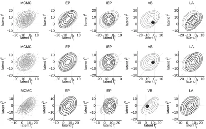
are shown. The EP approximation agrees reasonably well with the MCMC samples. IEP under-estimates the latent uncertainty, especially near the training inputs because of the skewing effect of the likelihood. This seems to affect more the predictive probabilities of the training points in Figure 5(b), which effect can also be seen in the previous example of Figure 2(a) further away from

the decision boundary near the input xi. Figure 6 shows that the VB method underestimates the

latent uncertainty. The independence assumption of VB leads to an isotropic approximate distribu-tion, and although the predictive probabilities for the training cases are somewhat consistent with MCMC, the predictions on the test data are less accurate (plots (c) and (h) in Figure 5). Note that the specific hyperparameter values are not optimal for VB, and these values are not supported by the marginal likelihood approximation of VB either, as will be visualized later in this section. The LA approximation captures some of the dependencies between the latent variables associated with

different classes, but the joint mode offis a poor estimate for the true mean, which causes

inaccu-rate predictive probabilities (plots (d) and (i) in Figure 5). The VB mean estimate is also closer to LA than MCMC, although LA uses a different observation model.

Kuss and Rasmussen (2005) and Nickisch and Rasmussen (2008) discussed how a large value of

the magnitude hyperparameterσ2_{can lead to a skewed posterior distribution in binary classification.}

In the multiclass setting, similar behavior can be seen in the marginal distributions as illustrated in

Figures 3 and 6. A largeσ2_{leads to a more widely distributed prior which in turn is skewed more}

−20 −10 0 10 −10 0 10 20 latent f i 1 latent f i 2 MCMC

−20 −10 0 10

−10 0 10 20 latent f i 1 latent f i 2 EP

−20 −10 0 10

−10 0 10 20 latent f i 1 latent f i 2 IEP

−20 −10 0 10

−10 0 10 20 latent f i 1 latent f i 2 VB

−20 −10 0 10

−10 0 10 20 latent f i 1 latent f i 2 LA

−20 −10 0 10

−20 −10 0 10 latent f i 1 latent f i 3 MCMC

−20 −10 0 10

−20 −10 0 10 latent f i 1 latent f i 3 EP

−20 −10 0 10

−20 −10 0 10 latent f i 1 latent f i 3 IEP

−20 −10 0 10

−20 −10 0 10 latent f i 1 latent f i 3 VB

−20 −10 0 10

−20 −10 0 10 latent f i 1 latent f i 3 LA

−10 0 10 20

−20 −10 0 10 latent f i 2 latent f i 3 MCMC

−10 0 10 20

−20 −10 0 10 latent f i 2 latent f i 3 EP

−10 0 10 20

−20 −10 0 10 latent f i 2 latent f i 3 IEP

−10 0 10 20

−20 −10 0 10 latent f i 2 latent f i 3 VB

−10 0 10 20

−20 −10 0 10 latent f i 2 latent f i 3 LA

Figure 6: Marginal posterior distributions for one training point with the true class label being 2

on the USPS 3 vs. 5 vs. 7 data. Each row corresponds to one of the latent pairs (f_i1,f_i2),

(f_i1,f_i3), and (f_i2,f_i3). The first column shows a scatter-plot of MCMC samples drawn from the posterior and estimated density contour levels which correspond to the areas that in-clude approximately 95%, 90% 75%, 50%, and 25% of the probability mass. The rest of the columns show the equivalent contour levels of the EP, IEP, VB, and LA approxima-tions (bold black lines) and the contour levels of the MCMC approximation (gray lines) for comparison. Note that the last column visualizes a different marginal distribution be-cause LA uses the softmax likelihood. The hyperparameters of the squared exponential

covariance function were fixed at log(σ2_{) =4 and log(l) =2 to obtain a non-Gaussian}

posterior distribution.

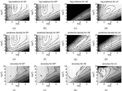
for demonstration purposes. However, usually the hyperparameters are estimated by maximizing the marginal likelihood. Kuss and Rasmussen (2005) and Nickisch and Rasmussen (2008) studied the suitability of the marginal likelihood approximations for selecting hyperparameters in binary classification. They compared the calibration of predictive performance and the marginal likelihood estimates on a grid of hyperparameter values. In the following, we extend these comparisons to multiple classes with the USPS data set, for which similar considerations were done by Rasmussen and Williams (2006) with the LA method.

The upper row of Figure 7 shows the log marginal likelihood approximations for EP, IEP, and

LA, and the lower bound on evidence for VB as a function of the log-lengthscale log(l) and

log-magnitude log(σ2_{)using the USPS 3 vs. 5 vs. 7 data. The middle row shows the log predictive}

accu-1 2 3 4 0 2 4 6 8 10 −400 −400 −400 −400 −300 −300 −300 −300 −220 −220 −220 −220 −190 −190 −190 −190 −170 −170 −170 −170 −160 −160 −160 −150 −150 −148.5

log evidence for EP

ln(l)

ln(

σ

2)

(a)

1 2 3 4

0 2 4 6 8 10 −400 −400 −400 −400 −300 −300 −300 −300 −220 −220 −220 −220 −190 −190 −190 −190 −170 −170 −170 −166 −166

log evidence for IEP

ln(l)

ln(

σ

2)

(b)

1 2 3 4

0 2 4 6 8 10 −700 −700 −700 −700 −500 −500 −500 −500 −500 −450 −450 −450 −450 −400 −400 −400

log evidence for VB

ln(l)

ln(

σ

2)

(c)

1 2 3 4

0 2 4 6 8 10 −400 −400 −400 −400 −300 −300 −300 −300 −220 −220 −220 −220 −190 −190 −190 −190 −170 −170 −170 −170 −160 −160

log evidence for LA

ln(l)

ln(

σ

2)

(d)

1 2 3 4

0 2 4 6 8 10 −300 −300 −300 −300 −200 −200 −200 −200 −125 −125 −125 −125 −100 −100 −100 −100 −80 −80 −80 −75 −75 −73.5 −73.5

predictive density for EP

ln(l)

ln(

σ

2)

(e)

1 2 3 4

0 2 4 6 8 10 −300 −300 −300 −300 −200 −200 −200 −200 −125 −125 −125 −125 −100 −100 −100 −100 −85 −85 −85 −80 −80 −80 −76.5 −76.5

predictive density for IEP

ln(l)

ln(

σ

2)

(f)

1 2 3 4

0 2 4 6 8 10 −400 −400 −400 −400 −300 −300 −300 −300 −300 −200 −200 −200 −200 −200 −150 −150 −150 −150 −150 −125 −125 −125 −125 −125 −110 −110 −110 −110 −110

predictive density for VB

ln(l)

ln(

σ

2)

(g)

1 2 3 4

0 2 4 6 8 10 −400 −400 −400 −400 −400 −300 −300 −300 −300 −300 −200 −200 −200 ₋₂₀₀ −200 −150 −150 −150 −150 −150 −125 −125 −125 −125

predictive density for LA

ln(l)

ln(

σ

2)

(h)

1 2 3 4

0 2 4 6 8 10 0.95 0.955 0.955 0.96 0.96 0.965 0.965 0.97 0.97 0.975 0.975 0.975 0.975 0.98 0.98 0.98 accuracy for EP

ln(l)

ln(

σ

2)

(i)

1 2 3 4

0 2 4 6 8 10 0.95 0.955 0.955 0.96 0.96 0.965 0.965 0.97 0.97 0.975 0.975 0.975 0.975 0.98 0.98 0.98 0.985

accuracy for IEP

ln(l)

ln(

σ

2)

(j)

1 2 3 4

0 2 4 6 8 10 0.95 0.955 0.96 0.965 0.97 0.975 0.98 0.985 0.985

accuracy for VB

ln(l)

ln(

σ

2)

(k)

1 2 3 4

0 2 4 6 8 10 0.95 0.95 0.955 0.955 0.96 0.96 0.965 0.965 0.97 0.97 0.97 0.97 0.975 0.975 0.975 0.98 0.98 0.98 0.985 0.985 0.985 0.985

accuracy for LA

ln(l)

ln(

σ

2)

(l)

Figure 7: Marginal likelihood approximations and predictive performances as a function of the

log-lengthscale log(l) and log-magnitude log(σ2_{)for EP, IEP, VB, and LA on the USPS 3}

vs. 5 vs. 7 data. The first row shows the log marginal likelihood approximations, the second row shows the log predictive densities in a test set, and the third row shows the classification accuracies in a test set.

racies. The marginal likelihood approximations and predictive densities for EP and IEP appear to be similar, but the maximum contour of the log marginal likelihood for IEP (the contour labeled with -166 in plot (b) of Figure 7) does not coincide with the maximum contour of the predictive density (the contour labeled with -76.5 in plot (f) of Figure 7), which is why a small bias can occur if the approximate marginal likelihood is used for selecting the hyperparameter values. With EP there is a good agreement between the maximum values in plots (a) and (e), and overall, the log predictive densities are higher than with the other approximations. The log predictive densities of VB and LA

are small where log(σ2)is large (regions whereq(f|

D

other hand, also the marginal likelihood approximations favor the areas of smaller log(σ2_)values.