http://www.sciencepublishinggroup.com/j/ijssam doi: 10.11648/j.ijssam.20180301.12
ISSN: 2575-5838 (Print); ISSN: 2575-5803 (Online)
Availability and Reliability Analysis for Dependent System
with Load-Sharing and Degradation Facility
Neama Salah Youssef Temraz
Mathematics Department, Faculty of Science, Tanta University, Tanta, Egypt
Email address:
To cite this article:
Neama Salah Youssef Temraz. Availability and Reliability Analysis for Dependent System with Load-Sharing and Degradation Facility. International Journal of Systems Science and Applied Mathematics. Vol. 3, No. 1, 2018, pp. 10-15. doi: 10.11648/j.ijssam.20180301.12
Received: May 22, 2018; Accepted: June 14, 2018; Published: July 13, 2018
Abstract:
In this paper, analysis of a system consists of two dependent components with degradation facility and load sharing is introduced. The system is considered to be consisted of two components connected in parallel and works dependently where the failure of any component affects the failure of the other one. In addition, it is assumed that there is a common failure between the two components. All failure and repair rates are assumed to be constant follow bivariate exponential distribution. Markov models are used to construct the mathematical model of the system. Analysis of the availability function and steady-state availability of the model is discussed. Reliability and mean time to failure for the system is introduced. A numerical example is given for illustration.Keywords:
Bivariate Exponential Distribution, Availability, Steady State Availability, Reliability, Mean Time to Failure, Markov Models, Load-Sharing Models, Degradation1. Introduction
Availability is the probability that the system is capable of conducting its required function when it is called upon given that it is not failed or undergoing a repair action. Reliability is the probability of a device performing its purpose adequately for the period of time intended under the operating conditions encountered (see Barlow and Prochan [1]). Failures can be defined in terms of degradation reaching a certain level (see for example Meeker and Escobar [2]).
Failure rate is the conditional probability that a device will fail per unit of time. The conditional probability is the probability that a device will fail during a certain interval given that it survived at the start of the interval (see Lawless [3]). A common cause failure is defined as a dependent failure in which two or more component fault states exist simultaneously, or within a short time interval, and are a direct result of a shared cause. Common cause failures are especially important for redundant components, and they may be classified in two main types: multiple failures that occur at the same time due to a common cause, and multiple failures that occur due to a common cause, but not necessarily at the same time (see Misra [4]).
In most cases, independence is assumed across the
components within the system which means that the failure of any component of the system does not affect the failure of another one in the system. However, if your system consists of multiple components sharing a load then the assumption of independence no longer holds true. If one component fails then the component(s) that are still operating will have to assume the failed unit's load. Therefore, the reliabilities of the surviving unit(s) will change. Calculating the system reliability is no longer an easy proposition.
Marshall and Olkin [6] introduced a bivariate exponential distribution by considering a reliability model in which two components fail separately or simultaneously upon receiving a shock that is governed by a homogeneous Poisson process. They derived the bivariate exponential distribution in several ways: the bivariate lack of memory property, shock models, a random sum model, and a minima model.
Freund [7] proposed a bivariate extension of the exponential distribution by allowing the failure rate of the surviving component to be affected after the failure of another component. Freund’s bivariate distribution is absolutely continuous and possesses the bivariate lack of memory property (see Bailey [8]). Freund’s model is one of the first to study bivariate distributions from reliability considerations, and it can be used to model load-sharing systems.
Huang and Xu [9] presented a general closed-form expression for the lifetime reliability of load-sharing k-out-of-n: G hybrid redundant systems. Temraz [10] introduced availability and reliability analysis for system with bivariate weibull lifetime distribution.
System failure is modeled in terms of the failures of the components of the system. Both the system and its components are often allowed to take only two possible states: a working state and a failed state. However, in many situations the units of the system can have finite number of states. In this paper, we consider that each component of the system has three states: up, degraded, and down. The transition from up state to degraded state represents a partial failure and the transition from degraded state to down (failed) state represents a complete failure.
El-Damcese and Temraz [11] presented a mathematical model for performing availability and reliability analysis of a parallel repairable system consisting of n identical components with degradation facility and common-cause failures.
Markov models are commonly used to perform reliability analysis of engineering systems and fault-tolerant systems. They are also used to handle reliability and availability analysis of repairable systems. First, we gave notations and several properties of stochastic processes. Next, we explore Markov chains focusing on criteria of recurrent/transient state, and long-run probabilities. We then discuss basic properties of the homogeneous Poison process, which is one of the most important stochastic processes. The discussion is then going to the continuous-time Markov chain, including the birth, the death, and the birth-death processes. It is not an easy task to solve the state equations. A number of solution techniques exist, such as analytical solution (see Rausand and Høyland [12]), Laplace-Stieltjes transforms (see Pukite [13]), numerical integration, and computer-assisted evaluation (see Block and Basu [14]).
In this paper, we present analysis for a system consists of two dependent units connected in parallel subject to load sharing and degradation facility. Markov models are used to construct a diagram and a mathematical model for a system. Availability analysis and steady state availability probability
for a system are discussed. Also, reliability and mean time to failure for a system is presented. A numerical example is introduced in order to show the results.
2. System Description
The system is considered to be consisted of two components connected in parallel and works dependently where the failure of any component affects the failure of the other one. In addition, it is assumed that there is a common failure between the two components. Each component of the system has two stages of failures. The first stage is the transition from up state to degraded state which represents a partial failure of the unit. The second stage is the transition from degraded state to failed state which represents a complete failure. Only complete failures are assumed to be repairable and the repaired unit is good as new. All failure and repair rates are assumed to be constant follow bivariate exponential distribution.
According to system description, the system will has nine states divided as follows:
The working states are: (0,0), (D,0), (0,D), (D,D), (F,0), (0,F), (D,F), (F,D), and the failed state is: (F,F).
2.1. Notations
The notations for the state probabilities are given as follows.
0,0 Probability that the system is up at time t
, 0 Probability that the first unit degraded and the
second unit is up at time t
0, Probability that the first unit is up and the
second unit degraded at time t
, Probability that both units degraded at time t
, 0 Probability that the first unit failed and the
second unit is up at time t
0, Probability that the first unit is up and the
second one failed at time t
, Probability that the first unit degraded and the
second one failed at time t
, Probability that the first unit failed and the
second one degraded at time t
, Probability that the system failed at time t
The notations for all possible transition rates between the states are defined as follows.
Transition rate from up state to degraded state for the first unit
Transition rate from up state to degraded state for the first unit after degradation of the second unit Transition rate from up state to degraded state for the first unit after failure of the second unit Transition rate from degraded state to failed state for the first unit
Transition rate from degraded state to failed state for the first unit after failure of the second unit Transition rate from up state to degraded state for the second unit
Transition rate from up state to degraded state for the second unit after degradation of the first unit Transition rate from up state to degraded state for the second unit after failure of the first unit Transition rate from degraded state to failed state for the second unit
Transition rate from degraded state to failed state for the second unit after degradation of the first unit
Transition rate from degraded state to failed state for the second unit after failure of the first unit Common transition rate from up state to degraded state for both units
Common transition rate from degraded state to failed state for both units
Repair rate for the first unit after failure
Repair rate for the first unit after it has failed and the second unit has degraded
Repair rate for the first unit after it has failed and the second unit has failed
Repair rate for the second unit after failure Repair rate for the second unit after it has failed and the first unit has degraded
Repair rate for the second unit after it has failed and the first unit has failed
Common repair rate for both units after common failure
2.2. System Availability
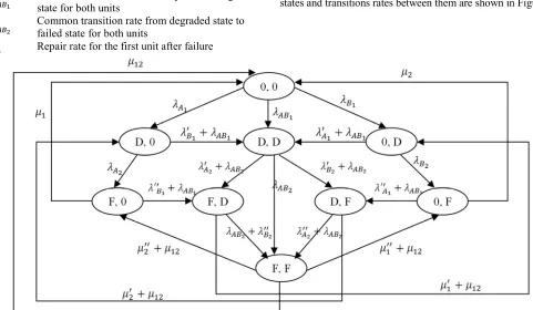
Continuous-time Markov chain is used to construct mathematical model for the system as follows. All possible states and transitions rates between them are shown in Figure 1.
Figure 1. Diagram for system of two dependent parallel units with degradation.
,
0,0 , 0 0, , (1)
,
, 0 , 0,0 (2)
,
0, , 0,0 (3)
,
3 , ! , 0 ! 0, 0,0 (4)
",
, 0 , , 0 (5)
,"
0, , 0, (6)
,"
", = − + + + , + + ! , + + + ! , 0
(8)
"," = − + + 3 , + + ! , + + + ! , + , (9)
The initial conditions for the system are given by #$%#&' ()$*%#)$+ = , 0,0 = 1 0 )%ℎ/01#+/ Equations from (1) to (9) form a system of first order differential equations which can be solved to obtain the state probabilities and the availability function can be calculated from the following sum of the probabilities of the working states. 2 % = 0,0 + , 0 + 0, + , + , 0 + + 0, + , + , (10)
2.3. Steady State Availability In Markov models, it is possible to go from one state to another one over a large long period of time. It can easily be shown that the limit #, 3 = lim→8 #, 3 always exists. One can get the steady state solutions by simply setting all the derivatives 9,: equal zero, and hence the system of differential equations will be reduce to an equivalent system of algebraic equations as follows. − + + 0,0 + , 0 + 0, + , = 0 (11)
− + + , 0 + + , + 0,0 = 0 (12)
− + + 0, + + , + 0,0 = 0 (13)
− + + 3 , + + ! , 0 + + + ! 0, + 0,0 = 0 (14)
− + + , 0 + + , + , 0 = 0 (15)
− + + 0, + + , + 0, = 0 (16)
− + + + , + + ! , + + + ! 0, = 0 (17)
− + + + , + + ! , + + + ! , 0 = 0 (18)
− + + 3 , + + ! , + + + ! , + , = 0 (19)
0,0 + , 0 + 0, + , + , 0 + 0, + + , + , + , = 1 (20)
The previous set of equations can be solved to obtain all possible probabilities. The steady state availability probability for the system can be obtained from the following sum. 2 = 0,0 + , 0 + 0, + , + , 0 + + 0, + , + , (21)
2.4. System Reliability Without Repair Reliability is defined as the probability that a part will last at least a specified time under specified experimental conditions (see Walpole et al. [15]). In order to obtain the reliability for the system, we set all repair rates equal to zero and then take Laplace transformation for the modified model and hence the following set of equations is obtained. + + + + ; 0,0 = 1 (22)
+ + + + ; , 0 − ; 0,0 = 0 (23)
+ + + + ; 0, − ; 0,0 = 0 (24)
+ + + + 3 ; , − + ! ; , 0 − + ! ; 0, − ; 0,0 = 0 (25)
+ ; 0, ; 0, 0 (27)
+ ; , ! ; , ! ; 0, 0 (28)
+ + + ; , ! ; , ! ; , 0 0 (29)
Reliability function of the system can be obtained by taking inverse Laplace transformation for all state probabilities and substituting in the following equation
< % => ?
; 0,0 ; , 0 ; 0, ; , ; , 0 ; 0, ; , ; , @ (30)
2.5. Mean Time to Failure
Mean time to failure (MTTF) is a measure of reliability for non-repairable systems. It is the mean time expected until the piece of equipment fails and needs to be replaced. MTTF is a statistical value and is calculated as the mean over a long period of time and a large number of units. Mean time to the system failure can be obtained from the following formula.
ABB lim;→ ; 0,0 ; , 0 ; 0, ; , ; , 0 ; 0, ; , ; , (31)
3. Numerical Example
We set failure and repair rates equal numerical values in the following table
Table 1. Values for failure and repair rates.
0.001 0.004 0.006 0.07
0.002 0.0045 0.0065 0.08
0.0025 0.0048 0.02 0.075
0.0015 0.0042 0.03
0.003 0.005 0.04
0.0035 0.0052 0.06
Substituting these values in the system of equations (1)-(9) and using Maple package to solve the system of differential equations, the availability function is obtained and the results are shown in Figure 2.
Figure 2. The availability function versus time.
Solving the system of equations (11)-(20) for the given data, steady state availability probability is computed from
equation (21) and the result is
A = 0.9949779728
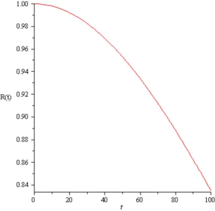
In order to find the reliability function, the set of equations (22)-(29) is solved and taking the inverse Laplace transformation for the results. Substituting in equation (30), reliability function is obtained and the result is shown in Figure 3.
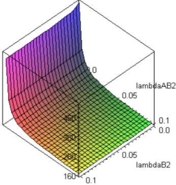
The results for the mean time to system failure are obtained by using equation (31). The results are illustrated in Figures 4 and 5.
Figure 4. The mean time to system failure versus and .
Figure 5. The mean time to system failure versus and .
4. Conclusion
In many situations in practical systems, there is dependence between the performances of the units constituting the system. Bivariate exponential distribution is suitable to model the life times of the dependent units. Degradation of system units is a generalization of the binary states of the system units. Markov model is a tool to analyze the availability and reliability of a system. It is not easy to
solve system of differential equations to find the state probabilities of the model and in this case, numerical solutions can be obtained instead of analytical solutions.
References
[1] Barlow R. E. and Prochan F., Statistical Theory of Reliability and Life Testing: Probability Models, Silver Spring, 1981. [2] Meeker W. Q. and Escobar L. A., Statistical Methods for
Reliability Data, Wiley, New York, 1998.
[3] Lawless J. F., Statistical Models and Methods for Lifetime Data, John Wiley & Sons, 1982.
[4] Misra K. B., Handbook of Performability Engineering, Springer-Verlag, London, 2008.
[5] Balakrishnan N. and Lai C. D., Continuous Bivariate Distributions, Springer, New York, 2009.
[6] Marshall A. W. and Olkin I., A Multivariate Exponential Distribution, Journal of American Statistical Association, 62, 30–44, 1967.
[7] Freund J. E., A Bivariate Extension of the Exponential Distribution, Journal of American Statistical Association, 56, 971–977, 1961.
[8] Bailey N. T. J., The Elements of Stochastic Processes, Wiley, New York, 1964.
[9] Huang L. and Xu Q., Lifetime Reliability for Load-Sharing Redundant Systems with Arbitrary Failure Distributions, IEEE Transactions on Reliability, 59, 2, 2010.
[10] Temraz, N. S., Availability and Reliability Analysis for System with Bivariate Weibull Lifetime Distribution, International Journal of Scientific & Engineering Research, 8(2), 376-389, 2017.
[11] El-Damcese M. A. and Temraz N. S., Analysis for Parallel Repairable System with Degradation Facility, American Journal of Mathematics and Statistics, 2(4), 70-74, 2012. [12] Rausand M. and Høyland A., System Reliability Theory:
Models, Statistical Methods, and Applications, Wiley, Hoboken, 2004.
[13] Pukite P. and Pukite J., Modeling for Reliability Analysis, IEEE, New York, 1998.
[14] Block H. W. and Basu A. P., A Continuous Bivariate Exponential Extension, Journal of American Statistical Association, 69, 1031–1037, 1974.