The Continuous Finite Element Methods for a Simple Case of Separable Hamiltonian Systems

Published online March 4, 2015 (http://www.sciencepublishinggroup.com/j/acm) doi: 10.11648/j.acm.20150402.12

ISSN: 2328-5605 (Print); ISSN: 2328-5613 (Online)

The Continuous Finite Element Methods for a Simple Case

of Separable Hamiltonian Systems

Qiong Tang

1, *

, Luohua Liua

1

, Yujun Zheng

2

1

College of Science, Hunan University of Technology, Zhuzhou, Hunan, P.R. China

2

Department of mathematics and Computational Science, Hunan University of Science and Engineering, YongZhou, Hunan, P.R. China

Email address:

[email protected] (Qiong Tang), [email protected] (Luohua Liua), [email protected] (Yujun Zheng)

To cite this article:

Qiong Tang, Luohua Liua, Yujun Zheng. The Continuous Finite Element Methods for a Simple Case of Separable Hamiltonian Systems.

Applied and Computational Mathematics. Vol. 4, No. 2, 2015, pp. 39-46. doi: 10.11648/j.acm.20150402.12

Abstract:

Combined with the characteristics of separable Hamiltonian systems and the finite element methods of ordinary

differential equations, we prove that the composition of linear, quadratic, cubic finite element methods are symplectic integrator to separable Hamiltonian systems, i.e. the symplectic condition is preserved exactly, but the energy is only approximately conservative after compound. These conclusions are confirmed by our numerical experiments.

Keywords:

Separable Hamiltonian Systems, Finite Element Methods, Composition Methods, Symplectic Integrator

1. Introduction

Hamiltonian system has two important properties: conservation and symplecticity. Traditional algorithms, such as classical R-K method , Adams method etc are nonsymplectic, eventually induce distortion. It is important to construct discrete algorithms which preserve these basic properties. H(q, p) = T(p) + V (q) is a simple case of separable Hamiltonian system. This kind of system is universal in chemical and physical modeling. Numerical computation method have good feature in terms of the ”kinetic T(p)+potential V (q)” form of the energy, many implicit symplectic difference scheme become explicit. K. Feng, M. Z. Qin, B. Leimkuhler, S. Reich, J. E. Marsden[1,2,3,4,5,6] et al. proved that composition of symplectic separable Hamiltonian is symplectic separable and constructed high order explicit symplectic difference methods. B. Leimkuhler, S. Reich et al.[6] utilize the wedge product and composition method proved Euler-A, Euler-B and the second-order Stormer-Verlet methods are canonically symplectic. Symplectic difference scheme constructed by symplectic geometry algorithm can maintain the basic characteristic of the system, and has particular superiority in relation to long -term tracking stability ability, but only obtains approximate energy conservation for nonlinear Hamiltonian system.

Utilizing the continuous finite element methods to study Hamiltonian system also has better properties. W. X. Zhong [7] et al. studied the linear finite element matrix to linear

vibrational equation with constant coefficients and proved that it maintained symplectic structure automatically. C. M. Chen et al. proved that applying m-th degree continuous finite element algorithm to Hamiltonian systems can obtain energy conservation, the linear and quadratic element are approximat -ely symplectic methods which have the accuracy of third and fifth order to their symplectic structure to nonlinear Hamiltoni -an systems respectively, and it is a symplectic algorithm for linear Hamiltonian systems [8,9].

In this paper, we utilize continuous finite element methods of ordinary differential equation and composition methods[1] to prove that the linear, quadratic, cubic continuous finite

element methods are symplectic integrator for separable Hamiltonian systems and the symplectic condition is preserve -d exactly, but the energy is only approximately conservative after compound. The numerical experiments are identical with theoretical analysis.

2. Continuous Finite Element Methods of

Ordinary Differential Equation

Consider the first-order ordinary differential equation with initial value in the interval K = [0,T]:

0

partition of K, and cell

I = (t ,t

j j j+1

), h = t

j j+1

-t ,

j j

h = max h ,

h

_j

≥

ch, 0

≤ ≤

j

N-1.

The constant number

c is independent of j and h. We define the m-th degree continuous finite element space in this partition as:

{

( ),

_j

}.

h

m I

S

=

ω ω

∈

C K

ω

∈

P

where

P

m is a m-th degree polynomial. In cell

I

j , m-th degree polynomial has m+1 degrees of freedom. It is an initial value problem, and we has already known the initial value

U t

( )

j in

I

j, so it has only m degrees freedom. Define m-th degree continuous finite element

U

∈

S

hto satisfy [10,11]:

j

m-1 0

I

(U -f(t,U))vdt=0,v

′

∈

P , (0)

U

=

u

.

∫

(2.2)

i.e., in cell

I

j, it is orthogonal to arbitrary Pm−1. Taking

h

S

ω

∈

, then its derivate ω′∈ Pm 1－ . In practical computation,

we can obtain equation set by taking

v = (t

－

t ) ,

_j i i =0, 1,

2,…,m − 1.

Lemma 1 [11] :The m-th degree continuous finite element for ordinary differential equation has super convergence in cell

t

j:

2m

j m+1,

(u - U)(t ) = O(h

) || u ||

_∞

.

(2.3) We take finite dimension autonomous Hamiltonian H(q, p) canonical systems

p q t=0 0 t=0 0

q = H ,p = -H ,q| = q ,p| = p .

′

′

(2.4)

Where T T

1 2 n 1 2 n

q = (q , q ,..., q ) ,p = (p , p ,...,p ) , matrix transpose is defined by ’T’. In applications to mechanical systems, q represents the generalized coordinate, p represents the canonical momentum and H represents the systems’s energy.

Let T

z =[q,p] , (2.4) can be written as

z 0 0

z =JH ,

′

z

_t=

=

z

.

(2.5)

Where n

0

J =

, I

0

n

n

I

I

−













is the n order unit matrix,

T

z q p

H =[H ,H ] .

According to (2.2),(2.5) and the linear element

j j+1

1-x

1+x

Z =

Z +

Z

,x

[-1,1]

2

2

∈

,we get the specific

calculation format of the linear continuous finite element as follow:

1

j+1 j ₁

Z -Z

( )

,

2

j

z

h

J

H Z dx

−

=

_∫

　j=0,1,...,N-1.

(2.6)

The specific calculation format of the quadratic continuous finite element is:

1

j+1 ₁

1

j+1 1 ₁

j+ 2

Z ( ) ,

2

5 2 1

Z Z ( )( 1) ,

6 3 6 4

j

j z

j

j z

h

Z J H Z dx

h

Z J H Z x dx

−

−

− =

− − = +

∫

∫

　　

(2.7)

Take 1 j j+

2

1 Z = Z(t + )

2hj

= , and the quadratic element

2 2

2

j 1 j+1

j+ 2

x x

Z = Z +(1-x )Z Z ,x [-1,1],

2 2

x x

− +

+ ∈ we can

solve the value

Z , j = 0, 1, ...,N-1

j+1 at each node step by

step.

In order to keep energy conservation, we utilize high accuracy numerical integration such as at least m + 1 point of the Gaussian quadrature formula to the m-th degree continuous finite element at the right of equation (2.6) and (2.7). From the above equation set , we can obtain a linear equation set of 1

j+ 2

Z

_and

j+1

Z

to linear Hamiltonian systems, nonlinear equation set of 1

j+ 2

Z

_and

j+1

Z

to nonlinear Hamiltonian systems, which can only definite the value

Z

j+1

when h is small.

According to (2.2), define equation set’s m-th degree continuous finite element

Z =[Q P]

T of z and it satisfies orthogonal relation:

j

z 0

I (Z'-JH ) 'v dt=0, (0)Z = z.

∫

(2.8)

Taking

v =[Q,P]

T, we obtain:

j j

p q

I I

0 0

(Q'-H ( , )) ' 0, (P'+H ( , )) ' 0, (0) (0) .

Q P P dt Q P Q dt

Q q P p

= =

= =

∫

　

∫

　

，

(2.9)

The second equation minus the first equation of (2.9), we can prove :

j j

q p

I I

d

(H

' H

')

H(Q,P)

0.

dt

Q

+

P dt

=

dt

=

∫

∫

(2.10)

Hence, at each nodes

t

j, we prove that:

j j j-1 j-1 0 0

H(Q(t ),P(t )) = H(Q(t ), P(t )) = ... = H(q ,p ).

Lemma 2[8]: Applying arbitrary degree continuous finite element to solve Hamilton equation, it maintains energy conservation.

Definition 1 [12] : A smooth map Ψ on the phase space 2n

Jacobin Ψ_z(z) satisfies:

T

z z

(

Ψ

(z)) J

Ψ

(z) =J.

(2.11)

for all z in the domain of definition of Ψ.

The definition

(

Ψ

_z

(z)) J

T

Ψ

_z

(z) =J

is not always the most convenient approach to check the symplecticness of given map Ψ because the wedge product notation can be combined with implicit differentiation which makes it a powerful tool to verify symplecticness of an implicitly transformation Ψ.

Conservation of symplecticness under a transformation

^

1 2

= (q, p), = (q, p)

q

p

∧

Ψ Ψ can be expressed as

^

d

q

d =dq

p

dp.

∧

∧ ∧

Definition 2 [6] A numerical method is symplectic integrator if the symplecticness condition

j+1 j+1 j j

dq

∧

dp

= dq

∧

dp

is preserved exactly.

Given two maps 1 n n

: R

R

Ψ

→

and 2 n n

: R

R

Ψ

→

with compatible range and domain, we define their composition _Ψ2 _Ψ1 _by

_[

Ψ Ψ

2 1

_{](z) =}

Ψ Ψ

2

₍

1

_(z))

for all n

z

∈

R

.

Lemma 3 [12] Linear combination of symplectic separable Hamiltonians is symplectically separable.

Utilizing Definition 2 and Lemma 3, B. Leimkuhler, S. Reich prove the Lemma 4 as follow.

Lemma 4[6]: Euler-A and Euler-B methods of a mechanical Hamiltonian

H(q,p)

are canonically symplectic with first-order accuracy.

The symplectic Euler-A method is

j+1 j j p j+1 j j+1 j j q j+1 j

q

= q + h

∇

H(q

, p ), p

= p - h

∇

H(q , p )

.

The symplectic Euler-B method is

j+1 j j p j j+1 j+1 j j q j j+1

q

= q + h

∇

H(q , p ), p

= p - h

∇

H(q , p

)

.

Therefore, Euler-A and Euler-B methods are explicit schemes to separable Hamiltonian systems

H(q, p) = T(p) + V (q)

.

3. Keep Symplectic Integrator for

Separable Hamiltonian Systems

Consider separable Hamiltonian systems:

t z 0

z = JH (z), z(0) = z .

(3.1)

Where

H(q, p) = T(p) + V (q)

. The form of the energy function suggests a natural splitting into kinetic energy

1

H (p) = T(p)

and potential energy

H (q) = V (q)

2 . The

differential equations corresponding to

H (q) = V (q)

2 can

be written as

d

d

0,

( )

dt

q

=

dt

p

= −∇

q

V q

(3.2)

The equations are completely integrable, since q is constant along solutions and p therefore varies linearly with time. Thus

1

H (p) = T(p) is similar.

3.1. The Linear Element

In the interval

I

j, m-th degree continuous finite element Z

satisfies :

j

t 1 0

I

(Z

−

JH Z vdt

z

( ))

=

0,

v

∈

P

m−

, (0)

Z

=

z

.

∫

　

　

(3.3)

We consider the linear element of the potential energy

H

2,

take m = 1, then

v

∈

P

0, obtain

j j

I I

dQ

dP

0,

( ) .

dt

dt

j

q I

dt

=

dt

= − ∇

V Q dt

∫

　

∫

∫

　

(3.4)

where the linear element of q is j+1 j 1

j j+1 j+1 j

t-t

t-t

Q =

t -t

Q

j

+

t

-t

Q

j+ ,

and it is similar to p.

Integrate the first equation of (3.4) in I , we can obtain j

j+1 j

Q

= Q

, then j+1 j 1

j j+1 j+1 j

t-t

t-t

Q =

t -t

Q

j

+

t

-t

Q

j+

=

Q

j in

interval I , So the second equation of (3.4) can be written as j

j

j+1 j _I j

P = P -

∫

∇

_q

V Q dt

( )

=

P -

h

_j

∇

_q

V Q

(

_j

)

_{. So the linear}

element of the potential energy H flow map is 2

h,V

([ ])

[

]

( )

q

q

q

p

h

V q

p

Ψ

=

− ∇

　

(3.6)

Similarly, the differential equations corresponding to

H

1can be written as

d

d

( ),

0.

p

q

T p

p

dt

= ∇

dt

=

(3.7)

Utilize the linear element,

j j

I I

dP

dQ

0,

( )

dt

dt

j

p I

dt

=

dt

=

∇

T P dt

∫

　

∫

∫

(3.8)

Integrate the first equation of (3.8) in Ij, we can obtain

j+1 j

P = P

, then j+1 j 1

j j+1 j+1 j

t-t

t-t

P=

j

I , the second equation of (3.8) can be written as

j

j+1 j _I j

Q

= Q +

∫

∇

_p

T P dt

( )

=

Q +

h

_j

∇

_p

T P

(

_j

).

　

(3.9)

So the linear element of the kinetic energy H flow map is 1

h,T

( ) ([ ])q [q h pT p ]

p p

+ ∇

Ψ = 　. (3.10)

Now consider the composition of these two maps

h,T h,V

= .

Ψh,H Ψ Ψ (3.11) Applying this map to a point of phase space

(q , p )

j j , we

first compute a point

_ _

( q , p )

,

_ _

q=q_j, p= p_j− ∇h_{j q}V q( _j). (3.12) Next, apply

Ψ

_{h T,} to this point, i.e.,

_ _ _

j+1 j+1

q = + ∇q hj pT(p), p =p.　 (3.13) These equations can be simplified by the elimination of the intermediate values, so

j+1 j+1 j+1

q =q_j+ ∇h_{j p}T(p ), p = p_j − ∇h_{j q}V q( _j).　 (3.14)

It is evidently the Euler-B method of a mechanical Hamiltonian.

If we consider this form composition of these two maps

h,H= h,V h,T

Ψ Ψ Ψ , then qj+1=q +hj j∇p T(p )j ,

j+1 j j q j+1

p = p -h

∇

V (q

)

. It is obviously the Euler-A method of

a mechanical Hamiltonian.

Combine Lemma 3, 4, we can prove the following theorem 1.

Theorem 1 The composition of linear element of the separable Hamiltonian systems is symplectic integrator, i.e. the symplectic condition dqj+1 ∧ dpj+1 = dqj ∧dpj is

preserved exactly.

3.2. The Quadratic Element

Here we consider the quadratic element for the separable Hamiltonian systems, take m = 2, then

v

∈

P

₁ , the differential equations corresponding to

H

₂ can be written as

j j

j j

j j

I I

q

I I

q

I I

dQ dQ

0, ( ) 0,

dt dt

dP

( ) , dt

dP

( ) ( )( ) .

dt

j

j j

dt t t dt

dt V Q dt

t t dt V Q t t dt

= − =

= − ∇

− = − ∇ −

∫

∫

∫

∫

∫

∫

　 (3.15)

Take transform hj t +tj j+1

t = x + ,

2 2 for

x

∈

[-1,1]

, the

quadratic element of q is

2

j 1 j+1

j+ 2

x(x-1) x(x+1)

Q= Q (1 )Q Q .

2 + −x + 2 From the first two equations of (3.15), we obtain

j+1 j j+1 j 1

j+ 2

Q

= Q , 5Q -Q = 4Q

_{, then} j+1 j 1

j+ 2

Q

= Q = Q

,

so

Q = Q

jin

I

j.

From the last two equations of (3.15) and

Q = Q

j in

I

j,

obtain j+1 1 j+

2

P

(

), P

(

),

2

j

j j q j j q j

h

P

h

V Q

P

V Q

=

− ∇

=

−

∇

The quadratic element of the potential term H flow map is 2

h,V

([ ])

[

].

( )

j q

q

q

p

h

V q

p

Ψ

=

− ∇

　

(3.16)

Similarly, the differential equations corresponding to

1

H

can be written as

j j

j j

j j

I I

p

I I

p

I I

dP

dP

0,

(

)

0,

dt

dt

dQ

( ) ,

dt

dQ

(

)

( )(

)

dt

.

j

j j

dt

t

t dt

dt

T P dt

t

t dt

T P t

t dt

=

−

=

= ∇

−

= ∇

−

∫

∫

∫

∫

∫

∫

　

(3.17)

From the first two equations of (3.17), we obtain j+1 j j+1 j 1

j+ 2

P = P , 5P -P = 4P ,

then j+1 j 1 j+

2

P = P = P , so

j

P = P in I . j

From the last two equations of (3.17) andP = P inj Ij, obtain j+1 1

j+ 2

Q ( ), Q ( ),

2

j

j j p j j p j

h Q h T P Q T P

= + ∇ = + ∇

The quadratic element of the potential term H1 flow map

is

h,T

( )

([ ])

q

[

q

h

p

T p

].

p

p

+ ∇

Ψ

=

　

(3.18)

Now we consider the composition of these two maps

h,H h,T h,V

Ψ = Ψ Ψ 　 (3.19) ApplyingΨ_h,Vthis map to a point of phase space(q , p ),j j

_ _

, ( ).

q

=qj

p

= pj − ∇hj qV qj 　

(3.20)

Next, applyΨh,T to this point

_ _

( ,

q p

), i.e.

_ _ _

1

q

( ),

p

1

p

.

j j p j

q₊ = + ∇h T p₊ = 　 (3.21)

These equations can be simplified by the elimination of the intermediate values, then

1

(

1

),

1

(

)

j j j p j j j j q j

q

₊

=

q

+ ∇

h

T p

₊

p

₊

=

p

− ∇

h

V q

. (3.22) It is evidently the Euler-B method of a mechanical Hamiltonian.

If we consider this form composition of these two maps

h,H

=

h,V h,T

Ψ

Ψ

Ψ

, and therefore

q

j+1

=q +h

j j

∇

p

T p

(

j

),

1

(

1

).

j j j q j

p

₊

=

p

− ∇

h

V q

₊ It is similarly the Euler-A method of a mechanical Hamiltonian.

Combine Lemma 3, 4, we can prove the following theorem 2.

Theorem 2 The composition of quadratic element of the separable Hamiltonian systems is symplectic integrator, i.e. the symplectic condition

dq

j+1

∧

dp

j+1

= dq

j

∧

dp

j is

preserved exactly.

3.3. The Cubic Element

We consider the cubic element for the separable Hamiltonian systems, take m = 3, then

v

∈

P

₂ , the differential equations corresponding to

H

₂ can be written as

j j

j j j

j j

j j

I I

2

q

I I I

q I I 2 2 q I I dQ dQ

0, ( ) 0, dt dt

dQ dP

( ) 0, ( ) ,

dt dt dP ( ) ( )( ) , dt dP ( ) ( )( ) . dt j j j j j j

dt t t dt

t t dt dt V Q dt

t t dt V Q t t dt

t t dt V Q t t dt

= − = − = = − ∇ − = − ∇ − − = − ∇ −

∫

∫

∫

∫

∫

∫

∫

∫

∫

　 　 (3.23)

Take transform

t =

h

j

x +

t +t

j j+1

,

2

2

for

x

∈

[-1,1]

, the

cubic element of q is

j 1 j+ 3 2 j+1 j+ 3 -(3x+1)(3x-1)(x-1) 9(3x-1)(x-1)(x+1)

Q= Q Q

16 16

9(3x+1)(x+1)(x-1) (3x-1)(3x+1)(x+1)

Q Q .

16 16

+

− +

From the first three equations of (3.23), we obtain

j+1 j

Q =Q , j+1 j 1 2

j+ j+

3 3

7Q -Q = 3Q +3Q ,

j+1 j 1 2

j+ j+

3 3

47Q -2Q = 9Q +36Q , _then j+1 j 1 2

j+ j+

3 3

Q = Q =Q =Q , so

j

Q = Q

in

I

j.

From the last three equations of (3.23), we obtain j+1

j+1 1 2

j+ j+

3 3

j+1 1 2

j+ j+

3 3

P ( ), 7

P 3P 3P 4 ( ),

47P 2 9P 36P 20 ( ).

j j q j

j j q j

j j q j

P h V Q

P h V Q

P h V Q

= − ∇

− − − = − ∇

− − − = − ∇

(3.24)

Solving the equations, we obtain

j+1 1 j+ 3 2 j+ 3

P ( ),

P ( ),

3 2

P ( ).

3 j j q j

j

j q j

j

j q j

P h V Q h P V Q

h P V Q

= − ∇

= − ∇

= − ∇ 　

(3.25)

The cubic element of the potential term

H

2flow map is

h,V

([ ])

[

].

( )

j q

q

q

p

h

V q

p

Ψ

=

− ∇

　

(3.26)

Similarly, the differential equations corresponding to

H

₁can be written as

j j j

j j

j j

j j

I I I

p I I p I I 2 2 p I I 2

dP dP dP

0, ( ) 0, 0,

dt dt dt

dQ ( ) , dt dQ ( ) ( )( ) , dt dQ ( ) ( )( ) dt

(

)

.

j j j j j j

dt t t dt dt

dt T P dt

t t dt T P t t dt

t t dt T P t t dt

t

t

= − = = = ∇ − = ∇ − − = ∇ −

−

∫

∫

∫

∫

∫

∫

∫

∫

∫

　 (3.27)

From the first three equations of (3.27), we obtain j+1 j 1 2

j+ j+

3 3

P

= P = P

=

P

,

　

so

P = P

j in

I .

j

From the last three equations of (3.27) and

P = P

j in

I

j, we

obtain j+1 1 j+ 3 2 j+ 3

Q ( ),

Q ( ),

3

2

Q ( )

3

j j p j

j

j p j

j

j p j

Q h T P

h

Q T P

h

Q T P

= + ∇

= + ∇

= + ∇

The cubic element of the potential termH flow map is ₁

h,T

( )

([ ])

q

[

q

h

p

T p

].

p

p

+ ∇

Ψ

=

　

(3.28)

Now we consider the composition of these two maps

h,H h,T h,V

Ψ = Ψ Ψ 　 (3.29) ApplyingΨ_h,Vthis map to a point of phase space(q , p ), j j

we first compute a point

_ _

, ( ).

q

=qj

p

= pj− ∇hj qV qj 　 (3.30)

Next, applyΨh,T to this point

_ _

( , )

q p

, i.e.

_ _ _

1

q

( ),

p

1

p

.

j j p j

q+ = + ∇h T p+ = 　 (3.31)

These equations can be simplified by the elimination of the intermediate values, then

1

(

1

),

1

(

)

j j j p j j j j q j

q

₊

=

q

+ ∇

h

T p

₊

p

₊

=

p

− ∇

h

V q

. (3.32) It is evidently the Euler-B method of a mechanical Hamiltonian.

If we consider this form composition of these two maps

h,H

=

h,V h,T

Ψ

Ψ

Ψ

, then

q

j+1

=q +h

j j

∇

p

T p

(

j

),

1

(

1

).

j j j q j

p

₊

=

p

− ∇

h

V q

₊ It is similarly the Euler-A method of a mechanical Hamiltonian.

Combine Lemma 3, 4, we can prove the following theorem 3.

Theorem 3 The composition of cubic element of the separable Hamiltonian systems is symplectic integrator, i.e. the symplectic condition dqj+1 ∧ dp = dqj+1 j ∧dpj is

preserved exactly.

3.4. About Energy Conservation of Hamiltonian System

According to the above analysis of the low-order finite element methods, if we apply composition methods

1 2

h,H= h,H h,H

Ψ Ψ Ψ of separable Hamiltonian systems to the potential energy

H = V (q)

₂ , because of

Q

j+1

= Q

j then

2 j+1 2 j

H (Q

) = H (Q )

, Similarly, to the kinetic

energy

H = T(p)

₁ , because of

P = P

j+1 j then

1 j+1 1 j

H (P ) = H (P )

. It is identical with Lemma 2, namely

every flow map maintains energy conservation. Although every flow map maintains energy conservation, the composition method

Ψ

h,H

=

Ψ

h,H₁

Ψ

h,H₂ is symplectic and

fit for order 1[2], after the compounded energy is only approximately conservative.

If we utilize the finite element methods to separable Hamiltonian systems

H(q, p) =T(p) + V (q)

directly, i.e., using the formula (2.6),(2.7), they can keep energy conservation of Hamiltonian systems, but the linear and quadratic element are approximately symplectic methods which have the accuracy of third and fifth order to their symplectic structure

respectively[9]. These conclusions also verify the Ge-Marsde theorem[13]: most numerical methods can’t maintain the two properties: symplectic and energy conservative simultaneously in general.

4. Numerical Experiments of Finite

Element Methods for Separable

Hamiltonian Systems

Molecular dynamics provides a rich source for geometric integration[14]. Here we consider A B2 type molecule’s

Hamilton function:

2 2 2 2 1

1 2

2 2 1 2 2

2 2 1 2

H(q,p)=2p 5 ( 5 6.5) 4

0.5 (| | 1.5) | | ( ) ( ), ( )

.

p D D D

q q T p V q D q q

π π

−

−

+ + − + +

+ − + = + = +

It’s canonical differential equations are

1 2 1 2

1 2 1 2

dq

dq

dp

dp

,

,

,

.

dt

dt

dt

dt

H

H

H

H

p

p

q

q

∂

∂

∂

∂

=

=

= −

= −

∂

∂

∂

∂

Initial condition:

1(0) = 3, 2(0) = 1.5, (0) = 0,1 2(0) = 0,H(0) = 50.1951.

q q p p

Take step length h = 0.01, total number of steps 8

10

K

=

,

integral interval 6

T =h K= 10

×

. Finite element methods

about the composition of these two maps

h,H

=

h,V h,T

Ψ

Ψ

Ψ

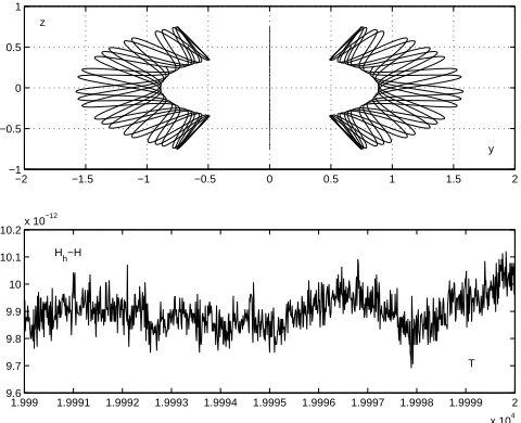
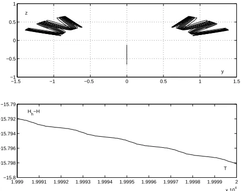
(FEMC), and directly utilizing the linear element(1FE), the quadratic element(2FE), the fourth-order classical R-K method(4RK) are considered to simulate A B₂ type molecule system respectively, the motion track and energy error

H -H

_h can be seen in figures 1-6.

From fig 1-6, FEMC’s solutions through the points of a region of phase space don’t be squeezed together over long time when total number of steps 8

K=10

, which reached the microscopic reaction dynamics research needed consideration of time 6

T = h K = 10

×

and can long preserve the structure

of phase space. 4RK isn’t symplectic difference format and phase space be squeezed into a smaller region only when integral steps 6

K = 2 10

×

. 1FE, 2FE can keep

A B

2 type

molecule’s motion trajectory stability for long time just like FEMC, energy error H -Hh only

-9

10

when 8

K = 10

.

From the above analysis, we conclude the main features of the continuous finite element methods to solve separable Hamiltonian systems H(q, p) = T(p) + V (q) : 1)Composition methods, the linear, quadratic, cubic element methods are symplectic integrator methods and can keep symplectic structure for the separable Hamiltonian system for a long time, but the energy is only approximately conservative after compound.

2)Directly utilizing the finite element method can keep energy conservation of Hamiltonian systems, but the linear and quadratic element are approximately symplectic methods which have the accuracy of third and fifth order to their symplectic structure to nonlinear Hamiltonian systems respectively.

It follows that finite element methods is a good method to study the Hamiltonian system for a long time.

−2 −1.5 −1 −0.5 0 0.5 1 1.5 2

−1 −0.5 0 0.5 1

0 1 2 3 4 5 6 7 8 9 10

−4 −2 0 2 4

y z

t H

h−H

Figure 1. FEMC, h=0.01, K= 3

10 , the initial points motion track and energy error plot.

−2 −1.5 −1 −0.5 0 0.5 1 1.5 2

−1 −0.5 0 0.5 1

9.9999 9.9999 9.9999 9.9999 9.9999 10 10 10 10 10 10

x 105 −4

−2 0 2 4

y z

5 H

h−H

Figure 2. FEMC, h=0.01, K= 8

10 , the last points motion track and energy error plot.

−2 −1.5 −1 −0.5 0 0.5 1 1.5 2

−1 −0.5 0 0.5 1

9.9999 9.9999 9.9999 9.9999 9.9999 10 10 10 10 10 10 x 105

−2 −1 0 1 2

y z

t H_h−H

Figure 3. FEMC, h=0.005, K= 8

2 10⋅ , the last 2000 points motion track and energy error plot.

−2 −1.5 −1 −0.5 0 0.5 1 1.5 2

−1 −0.5 0 0.5 1

9.9999 9.9999 9.9999 9.9999 9.9999 10 10 10 10 10 10

x 105 −6.8226

−6.8224 −6.8222 −6.822 −6.8218 −6.8216x 10

−9

erci

T H_h−H

Figure 4. 2FE, h=0.01,K= 8

10, the last 1000 points motion track and energy

error plot.

−2 −1.5 −1 −0.5 0 0.5 1 1.5 2

−1 −0.5 0 0.5 1

1.999 1.9991 1.9992 1.9993 1.9994 1.9995 1.9996 1.9997 1.9998 1.9999 2

x 104 9.6

9.7 9.8 9.9 10 10.1 10.2x 10

−12

z

y

T H

h−H

Figure 5. 1FE, h=0.01,K= 6

−1.5 −1 −0.5 0 0.5 1 1.5 −1

−0.5 0 0.5 1

1.999 1.9991 1.9992 1.9993 1.9994 1.9995 1.9996 1.9997 1.9998 1.9999 2

x 104 −15.8

−15.798 −15.796 −15.794 −15.792 −15.79

y z

T H_h−H

Figure 6. 4RK, h=0.01,K= 6

2 10⋅ , the last 1000 points motion track and energy error plot.

Acknowledgements

This research was supported by the National Natural Science Foundation of China (No: 11101136). The authors thank the anonymous reviewers for their useful comments that is helpful to the presentation of this paper.

References

[1] S.Blanes, “High order numerical integrators for differential equations using composition and processing of low order methods,”Appl. Numer. Math., vol.37,pp.289-306,2001. [2] K. Feng, M. Z. Qin, Symplectic Geometry Algorithm for

Hamiltonian systems. ZheJiang Press of Science and Technology, HangZhou, 2003,pp.10-220.

[3] K. Feng, M. Z. Qin, “Hamiltonian algorithms for Hamiltonian systems and a comparative numerical study,” Comput. Phys. Comm., vol.65, pp.173-187 ,1991.

[4] K. Feng, D. L. Wang, “On variation of schemes by Euler,” J. Comp. Math., vol.16, pp.97-106,1998.

[5] C. Kane, J. E. Marsden, M. Ortiz, “Symplectic-Energy-Momentum Preserving Variational Integrators,” J. Math. Phys., vol.40, pp.3353-3371 ,1999. [6] B. Leimkuhler, S. Reich, Simulating Hamiltonian Dynamics.

Cambridge Universty Press, Cambridge, 2004, pp.16–105.. [7] W. X. Zhong, Z. Yao, “Time Domain FEM and Symplectic

Conservation,” Journal of Mechanical Strength, vol.27,pp. 178-183 ,2005.

[8] Q. Tang, C. M. Chen, “Energy conservation and symplectic properties of continuous finite element methods for Hamiltonian systems,”.Appl. Math. and Comp.,vol. 181, pp.1357-1368 ,2006.

[9] Q. Tang, C. M. Chen, L. H. Liu, “Finite element methods for Hamiltonian systems,’ Mathematica Numerica Sinica, vol.31, pp.393-406 ,2009.

[10] C. M. Chen, Y. Q. Huang, High accuracy theory of finite element. Hunan Press of Science and Technology, Changsha, 1995,pp.70-150.

[11] C. M. Chen, Finite element superconvergence construction theory. Hunan Press of Science and Technology, Changsha, 2001,pp.80-158.

[12] K. Feng, Collected Works of Feng Kang. National Defence Industry Press, Beijing, 1995,pp.10-80.

[13] Z. Ge, J. E. Marsden, “Lie-Poisson integrators and Lie-Poisson Hamilton-Jacobi theory.,”Phys. Lett. A,vol. 133, pp.134-139 ,1998.