Grafting: Fast, Incremental Feature Selection by
Gradient Descent in Function Space
Simon Perkins [email protected]
Space and Remote Sensing Sciences Los Alamos National Laboratory Los Alamos, NM 87545, USA
Kevin Lacker [email protected]
Department of Computer Science University of California, Berkeley CA 94720, USA
James Theiler [email protected]
Space and Remote Sensing Sciences Los Alamos National Laboratory Los Alamos, NM 87545, USA
Editors: Isabelle Guyon and Andr´e Elisseeff
Abstract
We present a novel and flexible approach to the problem of feature selection, called grafting. Rather than considering feature selection as separate from learning, grafting treats the selection of suitable features as an integral part of learning a predictor in a regularized learning framework. To make this regularized learning process sufficiently fast for large scale problems, grafting operates in an incremental iterative fashion, gradually building up a feature set while training a predictor model using gradient descent. At each iteration, a fast gradient-based heuristic is used to quickly assess which feature is most likely to improve the existing model, that feature is then added to the model, and the model is incrementally optimized using gradient descent. The algorithm scales linearly with the number of data points and at most quadratically with the number of features. Grafting can be used with a variety of predictor model classes, both linear and non-linear, and can be used for both classification and regression. Experiments are reported here on a variant of grafting for classification, using both linear and non-linear models, and using a logistic regression-inspired loss function. Results on a variety of synthetic and real world data sets are presented. Finally the relationship between grafting, stagewise additive modelling, and boosting is explored.
Keywords: Feature selection, functional gradient descent, loss functions, margin space, boosting.
1. Introduction
to select a set of features before the underlying learning engine ever sees the data. Wrapper methods (Kohavi and John, 1997), do at least interact with an underlying learning engine, but they typically only communicate with it through brief summaries of performance, e.g. cross-validation scores. All the other information that the learning system might have gleaned from the data is usually ignored when choosing features.
More recently however, great efforts have been made to expand the applicability and robustness of general learning engines, and as a result, the distinction between feature selection and learning is beginning to look a little artificial. After all, are they not just two sides of the same overall task of learning a good model, given a set of training data described using a large number of features, and without using any special domain knowledge?
This observation motivates the approach presented in this paper, where we view feature selec-tion, whether for performance or pragmatic purposes, as part of an integrated criterion optimization scheme.
Section 2 of this paper presents the regularized risk minimization framework that forms the core of this scheme, and Section 3 introduces a fast, incremental method for finding optimal (or some-times approximately optimal) solutions, which we call grafting.1 Section 4 provides an empirical comparison of grafting with a number of other learning and feature selection techniques, and fi-nally, Section 5 draws conclusions and contrasts grafting with related work in stagewise additive modelling and boosting.
2. Learning to Select Features
In this paper, we view feature selection as just one aspect of the single problem of learning a map-ping based on training data described by a large number of features. At the core of this view is a common modern approach to machine learning, which can be described as regularized risk mini-mization. In the rest of this section, we review this approach, consider how it can be adapted to include feature selection, and explain why this might be a good idea.
2.1 Learning as Regularized Risk Minimization
First, a few definitions. We assume that we are trying to find a predictor function f(·) that maps feature2 vectors x of fixed length n, onto a scalar output value. If we have a binary classification problem then we derive an output label y∈ {−1,+1}with y=sign(f(x)). If we have a regression problem then we produce an output predicted value y= f(x). Since this is a machine learning paper, f(.)is derived, via a learning procedure, from a training set consisting of m randomly sampled(x,y) pairs drawn from the distribution we’re attempting to model.
We assume that f(·)is a member of a family of predictor functions that are parameterized by a set of parametersθ. We can specify a particular member of this family explicitly as fθ(·), but we will often omit the subscript for brevity. We want to come up with aθthat minimizes the expected risk:
R(θ) = Z
L(fθ(x),y)p(x,y)dx dy (1)
1. The name “grafting” is derived from “gradient feature testing”, for reasons that will become clear.
where L(f(x),y)is a loss function that specifies how much we are penalized for returning f(x)when the true target value is y; and p(x,y)is the joint probability density function for x and y. For classifi-cation problems the most common loss function is the misclassificlassifi-cation rate: L≡12|y−sign(f(x))|. In general we do not know p(x,y)in (1), so it is usually not possible to directly optimize that cri-terion with respect toθ. Instead, we usually work with the empirical risk Rempcalculated from the
training data, with the integral in (1) replaced by a sum over all data points. As is well known, directly optimizing the empirical risk can lead to overfitting, so it is common in modern machine learning to attempt to minimize a combination of the empirical risk plus a regularization term to penalize over-complex solutions. That is, we attempt to minimize a criterion of the form:
C(θ) = 1 m
m
∑
i=1
L(fθ(xi),yi) +Ω(θ) (2)
whereΩ(θ)is a regularization function that has a high value for “complex” predictors f .
2.1.1 LOSS FUNCTIONS FORCLASSIFICATION
In theory, we could simply use the error rate as the loss function in (2), but there are two main problems with this. First, this loss function almost inevitably leads to an optimization problem that is hard to solve exactly. Second, experience and theory have shown that we obtain robust and better generalizing classifiers if we prefer classifiers that separate the data by as wide a margin as possible. Discussion of this phenomenon, and many examples, can be found in Smola et al. (2000). We can usually improve generalization performance and make the criterion easier to optimize by choosing a loss function that encourages such large-margin solutions.
We define the margin for a classifier f on a single data point x with true label y∈ {−1,+1}to beρ=y f(x). The margin is positive if the point is correctly classified (the sign of f(x)agrees with the sign of y), and negative otherwise.
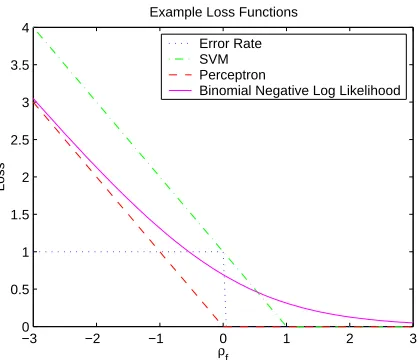
Many commonly used loss functions can be conveniently defined in terms of this margin. Fig-ure 1 illustrates a few of these.
In our classification work, we use the Binomial Negative Log Likelihood loss function (Hastie et al., 2001, p. 308):
Lbnll=ln(1+e−ρ)
This loss function is derived from a model that treats f(x)as the log of the ratio of the probability that y= +1 to the probability that y=−1.
The main value of this assumption is that it allows us to calculate p(x)≡p(y= +1|x) from f(x)using the following relation:
p(x) = e
f(x)
1+ef(x)
This loss function can also be readily generalized to a multi-class classification problem using the ideas of multi-class logistic regression (Hastie et al., 2001, pp. 95–100). That reference also contains a derivation of the loss function.
Lbnlldefines the BNLL loss for a single data point. It also useful to define the total loss over the
training set, also known as the empirical risk, which is the first term in (2):
LBNLL=
1 m
m
∑
−3 −2 −1 0 1 2 3 0
0.5 1 1.5 2 2.5 3 3.5 4
ρ f
Loss
Example Loss Functions
Error Rate SVM Perceptron
Binomial Negative Log Likelihood
Figure 1: Commonly used loss functions, plotted as a function of the margin ρ=y f(x). Shown are the “SVM” loss function: Lsvm=max(0,1−ρ); the perceptron criterion: Lper=
max(0,ρ); and the binomial negative log-likelihood: Lbnll=ln(1+e−ρ).
2.1.2 REGULARIZATION
Possibly the most straightforward approach to machine learning involves defining a family of mod-els and then selecting the model that minimizes the empirical risk. While this is certainly an often-used technique, it has two serious problems.
The first problem is that for certain combinations of model family, empirical risk function, and training data, the optimization problem can be unbounded with respect to the model parametersθ. For example, consider the linear model defined by:
f(x)≡
n
∑
i=1
wixi+b (3)
where w= (w1,...,wn)T is a vector of weights, xiis the i’th feature of the feature vector x, and b is
a constant offset. If the training data is linearly separable, then we can increase the magnitude of w indefinitely to reduce LBNLL.
The second problem is the well-known overfitting problem. Given a sufficiently flexible family of classifiers, it is often possible to find one that has a very low empirical risk, but that generalizes very badly to previously unseen data.
Both these problems can be tackled by adding a regularization term to the empirical risk. The regularization term (or regularizer) is a function of the model parameters that returns a high value for “unlikely” or complex models that are liable to generalize badly. By optimizing a sum of the regularizer and the empirical risk, we achieve a trade-off between model simplicity and empirical risk. If the balance is chosen appropriately then we can often improve generalization performance significantly compared with simple empirical risk minimization.
Given this parameter vector, we can define a commonly employed family of regularizers param-eterized by a non-negative integer q, and a vector of positive real numbersα:
Ωq(w) =λ p
∑
i=1
αi|wi|q (4)
Members of this regularizer family correspond to different kinds of weighted Minkowski norm of the parameter vector, and so Ωq is often referred to as an lq regularizer. Usually, we choose
αi∈ {0,1}so as to simply include or exclude certain elements of w from the regularization.3 The
essence of these regularizers is that they penalize large values of wiwhenαi>0.
It is easy to show that the solutions found by unconstrained minimization of (2) using an Ωq
regularizer are equivalent to those found by the following constrained optimization problem:
minimize 1 m
m
∑
i=1
L(f(xi),yi) (5)
s.t.
p
∑
i=1
αi|wi|q≤γ
There is a one-to-one (but not necessarily simple) correspondence between the parametersλand
γ. This alternative formulation is useful when we consider theΩ0regularizer.
The most interesting members of the family involve q∈ {0,1,2}. The following is a summary of the properties and peculiarities if these three regularizers.
Ω2 This regularizer is seen in ridge regression (Hoerl and Kennard, 1970), the support vector ma-chine (Boser et al., 1992, Sch¨olkopf and Smola, 2002) and regularization networks (Girosi et al., 1995). Those references give various justifications for this form of regularization. One reason for preferring it over otherΩqregularizers is that it is the only one which produces the
same solution under an arbitrary rotation of the feature space axes. The l2norm also makes the solution to (2) bounded. Asλis increased, the magnitudes of the elements of w will tend to decrease, but in general none will go to zero. The l2norm is a convex function of weights, and so if the loss function being optimized is also a convex function of the weights, then the regularized loss has a single local (and global) optimum.
Ω1 The l1-based regularizer is also known as the “lasso”. Tibshirani (1994) describes it in great detail and notes that one of its main advantages is that it often leads to solutions where some elements of w are exactly zero. Asλ is increased, the number of zero weights steadily in-creases. Unlike theΩ2regularizer, using the l1norm means that an arbitrary rotation of the feature axes in general produces a different solution, so the feature axes have special status with this choice of regularizer. Like theΩ2regularizer, this regularizer leads to bounded solu-tions. Similarly, the l1norm is a convex function of weights, and so if the loss function being optimized is also a convex function of the weights, then the regularized loss has a single local (and global) optimum.
Ω0 If we define 00≡0, then this contributes a fixed penalty αi for each weight wi6=0. If all αi
are identical, then this is equivalent to setting a limit on the maximum number of non-zero weights. The l0norm is, however, a non-convex function of weights, and this tends to make exact optimization of (2) computationally expensive.
2.2 Feature Selection as Regularization
If we have a mathematical expression for a model in which feature vector elements only ever appear with an associated multiplicative weight, then the process of feature selection amounts to producing a model in which only a subset of weights associated with features are non-zero. Of the regularizers described above,Ω0andΩ1lead to solutions with some weights set to exactly zero. But can they be justified in terms of the standard reasons for feature selection?
There are many motivations for feature selection, but we will consider two broad classes which generally encompass the reasons most commonly given.
2.2.1 PRAGMATIC MOTIVATIONS FORFEATURESELECTION
Often, the motivations for feature selection are pragmatic. We wish to reduce training time; reduce the time it takes to apply a learned model to new data; reduce the storage requirements for the model; or improve the intelligibility of the model. We can interpret all of these as either constituting a fixed penalty for including a feature in the model, or as a constraint on the maximum number of features in the model. For the simplest linear model case, where each feature appears in the model associated with just a single weight, then it is easy to see that both of these interpretations correspond to aΩ0 regularizer withαi>0 only where wiis the multiplicative weight on a feature. For more complex
models, where each feature might be associated with several weights, then we can handle this with a slightly modified version of theΩ0regularizer:
Ω0(w) =
n
∑
i=1
αiδi (6)
whereδi=maxj∈si(w
0
j), in which siis the set of weight indices associated with the i’th feature.
If different features carry different costs, for instance if some features are very expensive to compute, then we can adjust theαi associated with those features accordingly.
2.2.2 PERFORMANCE MOTIVATIONS FORFEATURESELECTION
The other common motivation for feature selection is to improve the generalization performance of our learned models. In general, the more feature dimensions a model includes, the greater its “capacity”, and hence the greater the tendency for it to overfit the training data — the so-called “curse of dimensionality”. But regularization techniques are intended to prevent overfitting, and the question arises: if we use regularization, do we need to do any additional feature selection? Or alternatively, can we achieve improved generalization performance by using a regularizer that encourages zero-weighted features in our model, such as theΩ1andΩ0regularizers?
0 2 4 6 8 10 12 0
0.05 0.1 0.15 0.2 0.25 0.3
Irrelevant features
Mean misclassification rate
σ=0.5
0 2 4 6 8 10 12
0 0.05 0.1 0.15 0.2 0.25 0.3
Irrelevant features
Mean misclassification rate
σ=1.0
Ω0 Ω1 Ω2
Unregularized Bayes Error
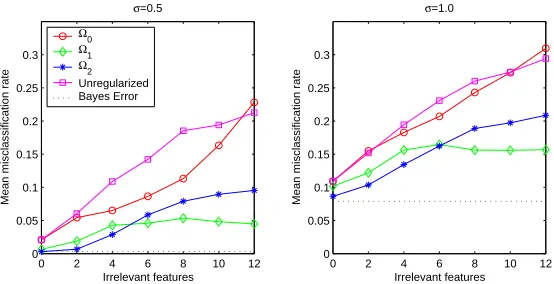
Figure 2: Comparison of different regularization schemes on a problem with varying numbers of irrelevant features and different optimal Bayes error.
features are irrelevant. Training sets with between 0 and 12 irrelevant features were generated, each containing 10 samples drawn from each class. We compared problems withσ=0.5 andσ=1.0. The former has a Bayes misclassification rate of 0.0035, the latter has a Bayes misclassification rate of 0.079. Test sets were generated in the same way, but with 1000 samples in each class. We used a linear model as in (3) which was trained by optimizing a regularized risk criterion (2), using the logistic regression loss function Lbnlland one of the threeΩqregularizers, or using no regularization.
ForΩ1andΩ2we used a gradient descent algorithm (Nelder and Mead, 1965), and forΩ0we used backward elimination (Kohavi and John, 1997), choosing to eliminate the feature that increased the loss function by the least at each step. This is a greedy procedure that may not produce the optimal answer, but exhaustive subset comparison was impractically slow. The regularization parameters (λ for theΩ1andΩ2regularizers,γfor theΩ0regularizer) were found by generating multiple instances of each problem and searching for the values that minimized the average misclassification rate.
Figure 2 compares the performance of the various regularizers as the number of irrelevant fea-tures is altered. For each problem type, 200 training and test sets were randomly generated. The plots show the mean test score for each type of regularizer, and for the two different values ofσ. For reasons of clarity, error bars indicating the standard error of the mean misclassification rate are not shown here, but they are small compared to the separation between the curves.
Both values ofσproduce qualitatively similar results. The unregularized and subset selection (Ω0) experiments perform worst, although subset selection does relatively better when the informa-tive features are well-separated in the lowσcase. Of the other two experiments, when most features are relevant, then Ω2 regularization slightly outperforms Ω1 regularization. But as the number of irrelevant features increases, Ω1 regularization takes the lead. Interestingly, when more than two-thirds of the features are irrelevant in this case, the test performance usingΩ1regularization seems to level off, while the performance usingΩ2regularization continues to degrade.
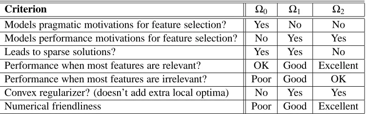
Criterion Ω0 Ω1 Ω2 Models pragmatic motivations for feature selection? Yes No No Models performance motivations for feature selection? No Yes Yes
Leads to sparse solutions? Yes Yes No
Performance when most features are relevant? OK Good Excellent Performance when most features are irrelevant? Poor Good OK Convex regularizer? (doesn’t add extra local optima) No Yes Yes
Numerical friendliness Poor Good Excellent
Table 1: Comparison of three differentΩqregularizers.
2.3 A Unified Optimization Criterion
We have argued that for a significant class of models, described by real-valued parameter vectors, many motivations for feature selection can be incorporated into a regularized risk minimization framework, using a suitable combination ofΩqregularizers.
Table 1 summarizes the different qualities of the three Ωqregularizers we have considered. In
general, we might want to use all three, which leads to the following optimization criterion:
C(w) = 1 m
m
∑
i=1
L(f(x),yi) +λ2
p
∑
i=1
α2,i|wi|2+λ1
p
∑
i=1
α1,i|wi|+λ0
n
∑
i=1
α0,iδi (7)
3. Grafting
We wish to find a minimum of (7), with respect to our model parameters. We now consider how this might be done, and introduce the grafting algorithm, as a fast way of getting to an optimal or approximately optimal solution, ifλ0orλ1is non-zero.
3.1 Direct Gradient Descent Optimization
Probably the most direct method of solution of (7) is to perform gradient descent with respect to the model parameters w, until a minimum is found. If we can compute the gradient of the loss function and the regularization term(s) with respect to these parameters, then we can use conjugate gradient or quasi-Newton methods. If not, then we can use a minimization method that doesn’t require gradient information, such as Powell’s direction set method. See Press et al. (1992, chap. 10) for overviews of these methods.
Unfortunately there are a number of problems with this approach. Firstly, the gradient descent can be quite slow. Algorithms such as conjugate gradient descent typically scale quadratically with the number of dimensions,4 and we are particularly interested in the domain where we have many features and so p is large. This quadratic dependence on number of model weights seems particularly wasteful if we are using the Ω0 and/or Ω1 regularizer, and we know that only some subset of those weights will be non-zero.
The second problem is that theΩ0andΩ1regularizers do not have continuous first derivatives with respect to the model weights. This can cause numerical problems for general purpose gradient descent algorithms that expect these derivatives to be continuous.
Finally, we have the problem of local minima. TheΩ2andΩ1regularizers are convex functions of the weights and so if the loss function being used is also a convex function of weights, then we have a single optimum. TheΩ0 regularizer on the other hand is not convex and introduces many local minima into the optimization problem.
3.2 Stagewise Gradient Descent Optimization
If we are using theΩ1orΩ0regularizer, and we suspect that the number N of non-zero weights in the final model is going to be much less than the total number of weights n, then a more efficient stagewise optimization procedure suggests itself. We call this algorithm grafting. The basic plan is to begin with a model in which almost all weights are at zero. At each iteration of the grafting pro-cedure, we use a fast gradient-based heuristic to decide which zero weight should be adjusted away from zero in order to decrease the optimization criterion by the maximum amount. We then perform gradient descent using that weight and any other non-zero weights in the model, and continue until no further progress can be made.
3.2.1 THEBASICGRAFTING ALGORITHM
For ease of presentation, we first consider the case whereλ0=0 in (7), butλ1andλ2are non-zero. We will return to the case whereλ06=0 later. At this stage, our discussion applies to a broad class of models and loss functions.
As described above, we assume that the model we are using is parameterized by a weight vector w. At any stage in the grafting process, the model weights are divided into two disjoint sets. Those weights wi∈
F
are “free” to be altered as desired. The remaining weights wi∈Z
(≡ ¬F
)are fixedat zero.
We also assume that the output of the model for a given training example is differentiable with respect to the model weights, i.e. we can calculate∂f(xi)/∂wj for an arbitrary feature vector xiand
and an arbitrary weight wj.
As explained below, after each grafting step (and before the first step) we minimize (7) with respect to the free weights, so before the k’th grafting step, we have:
∀i∈F ∂C
∂wi =0
During the k’th grafting step, we wish to move one weight from
Z
toF
. It seems sensible to select the weight which is going to have the greatest effect on reducing the optimization criterion C. The gradient of the criterion with respect to an arbitrary model weight wiis:∂C
∂wi =
1 m
m
∑
i=1
∂
L
∂f(xi)
∂f(xi)
∂wi
+2λ2α2,iwi+λ1α1,isign(wi)
= 1
m
m
∑
i=1
∂
L
∂f(xi)
∂f(xi)
∂wi
±λ1α1,i (8)
The contribution from theΩ2term disappears because wi=0 for all wi∈
Z
. Slightly more subtleis the replacement of sign(wi)with±1, which invites the question of what sign should be used, and
determining which weight, when adjusted in the appropriate direction, will decrease C at the fastest rate. Consider ∂LT OT/∂wi, the derivative of the total loss with respect to wi (this is just the first
term in the above expression). Suppose that ∂LT OT/∂wi >λ1α1,i. This means that ∂C/∂wi>0,
regardless of the sign of wi. In this case, in order to decrease C, we will want to decrease wi. Since
wistarts at zero, the very first infinitesimal adjustment to wiwill take it negative. Therefore for our
purposes we can let sign(wi) =−1. Similarly, if∂LT OT/∂wi<−λ1α1,i, then we can effectively
let sign(wi) = +1. Essentially, the effect of theΩ1 derivative is simply to reduce the magnitude of
∂C/∂wiby an amountλ1α1,i. The same argument shows that if|∂LT OT/∂wi|<λ1α1,i then it is not
possible to produce any local decrease in C by adjusting wi away from zero. This is the essence of
why theΩ1regularizer leads to solutions with zero-valued weights, and also provides the basis for one of the two stopping conditions discussed below.
At each grafting step, we calculate the magnitude of ∂C/∂wi for each wi∈
Z
, and determinethe maximum magnitude. We then add the weight to the set of free weights
F
, and call a general purpose gradient descent routine to optimize (7) with respect to all the free weights. Since we know how to calculate the gradient of∂C/∂wi, we can use an efficient quasi-Newton method. Weuse the Broyden-Fletcher-Goldfarb-Shanno (BFGS) variant (see Press et al. 1992, chap. 10 for a description). We start the optimization at the weight values found in the k−1’th step, so in general only the most recently added weight changes significantly.
Note that choosing the next weight based on the magnitude of∂C/∂wi does not guarantee that
it is the best weight to add at that stage. However, it is much faster than the alternative of trying an optimization with each member of
Z
in turn and picking the best. We shall see below that this procedure will take us to a solution that is at least locally optimal.3.2.2 INCORPORATING THEΩ0REGULARIZER
Use of the Ω0 regularizer means that transferring a weight wi from
Z
toF
incurs a penalty ofλ0α0,iδi. This fixed penalty makes it substantially harder to determine which weight is the most
promising one to transfer to
F
.5 The heuristic we use in this case is based upon the empirical observation that in a sequence of grafting steps, the magnitude of the most recently added weight inF
typically decreases monotonically. This allows us to estimate an upper limit on the magnitude of the weight we are about to add, which in turn means we can roughly estimate a bound on the change in C which will result from adding a weight wiin the grafting step after a weight wj was added:∆C(wi)≥λ0α0,iδi−wj
∂LT OT
∂wi
−λ1α1,i−λ2α2,iwj
(9)
Picking the best weight to add then amounts to choosing wi∈
Z
that minimizes (9). Note thatifλ0=0 and ∀{wi,wj} ⊂
Z
:α2,i =α2,j, then this heuristic is equivalent to the simple heuristicpreviously discussed.
3.2.3 STOPPING CONDITIONS
If only the Ω2 regularizer is being used, then in general the model will contain no zero-valued weights, and the grafting procedure will not terminate until
Z
is empty. In this case there is no advantage in using grafting over full gradient descent optimization.5. One exception is when all weights inZincur the sameΩ0penalty, as is the case with a simple linear model where
If we are using theΩ1regularizer, then we can reach a point where: ∀wi∈
Z
∂LT OT
∂wi
≤λ1α1,i
At this point it is not possible to make any further decrease in C by either moving a weight from
Z
toF
, or by adjusting any weights inF
and so we are at a local (and perhaps global) minimum, and can terminate the grafting procedure.If we are using theΩ0 regularizer, then we may reach a point where C increases after adding wi to
F
. We must then set wi to zero, remove it fromF
, and undo the last optimization step (itis convenient to keep a copy of the previous model around in order to avoid an extra optimization step). We then have a choice. It is possible that a different choice of wi might lead to a decrease in
C, so we could try the optimization step again with the wi associated with the next lowest value of
∆C(wi). This cycle could be repeated until all remaining weights in
Z
have been eliminated, andthe algorithm then terminates. Alternatively we can just terminate the algorithm the first time this happens, recognizing that with theΩ0 regularizer, our solution will be a greedy approximation to the optimal solution at best. The latter approach is the one we recommend in most cases.
3.2.4 OPTIMALITY
If we have a convex loss function (as a function of weights) and are using just theΩ2 and/or Ω1 regularizers (which are themselves convex functions of the weights), then there is only one minimum of (7). Examination of the stopping conditions above reveal that the grafting algorithm is guaranteed to stop at a local optimum, and so grafting is guaranteed to find the global optimum in these cases.
As we have seen by now, use of the Ω0 regularizer makes it much harder to find an optimal solution. The grafting procedure with non-zeroλ0amounts to a greedy heuristic forward subset se-lection method, which sacrifices optimality in return for fast learning. Whether this is good enough for the problem at hand depends on the situation.
One should note however, that asλ0is made smaller and smaller relative toλ1, then the chances of ending up in a sub-optimal situation decrease. Hence we are inclined to makeλ0fairly small in most cases.
3.2.5 COMPUTATIONAL COMPLEXITY
We have claimed that grafting is substantially faster than full gradient descent. We will now exam-ine this claim more carefully. If there are p weights in our weight vector, then full gradient descent requires some multiple of p line minimizations to optimize our criterion, let’s say cp minimiza-tions.6 Determining the direction requires p derivatives∂C/∂w
i to be computed. The computation
of each derivative is dominated by the computation of∂LT OT/∂wi, which is simply a weighted sum
of m simple derivatives∂f(xj)/∂wi. The line minimizations themselves require a few O(m)
func-tion evaluafunc-tions, but if p is large, then this is a minor contribufunc-tion. If we denote the time taken to calculate one simple derivative asτ, then the total time taken for full gradient descent is≈cmp2τ.
Under grafting we will select some number s weights before the algorithm terminates. Since we select one weight at each grafting step we take s steps. The k’th step consists of two phases. First we evaluate ∂C/∂wi for each of the (p−k) weights in
Z
. As noted above, the derivativecalculation takes mτ, and so the time devoted to gradient testing over s steps is ≈mspτ. The
second phase involves optimizing with respect to the k free weights. At most this might take ck line minimizations, but it should take less than this since most of the free weights will be close to their optimal values. To compensate for using a constant c that is probably too high here, we again ignore the time taken for the line minimizations themselves (some small multiple of mτ). Therefore the time taken for optimization at the k’th step is≈cmk2τ. Over s steps, this is≈13cms3τ. Putting this together the total grafting run time is≈(msp+13cms3)τ. If we assume that s p then it is clear that the grafting algorithm should be substantially quicker than the≈cmp2τrequired for full gradient descent. Also note that the full gradient descent algorithm has to deal with discontinuities in the gradient which can slow it down significantly. By keeping zero-valued weights out of the optimization steps, grafting avoids this difficulty.
3.2.6 NORMALIZATION
In order to make the gradient magnitude heuristic a fair comparison, it is usually important to normalize all features so that they have approximately the same scale. Before we begin, we linearly scale all feature vectors so that each feature has a mean value of zero and has a standard deviation of one. It is of course important to scale testing data using the same scaling parameters derived from the training data.
3.3 Grafting Examples
It is helpful to illustrate the grafting algorithm in more detail for some particular models and loss functions. Here we will concern ourselves only with binary classification problems and so a suitable loss function to use is the binomial negative log likelihood Lbnll. For simplicity, we will also assume
onlyΩ1andΩ0regularization are used, and that allα1,i∈ {0,1}.
3.3.1 LINEARMODEL
We first consider linear models with n+1 weights, of the form:
f(x) =
n
∑
i=1
wixi+w0
If we define the margin for a given training pair(xi,yi)asρi=yif(xi), then the following is the
regularized optimization criterion:
C(w) = 1 m
m
∑
i=1
(1+e−ρi) +λ
1
n
∑
i=1
|wi|+λ0s (10)
where s is the number of selected features. Note that the constant offset term w0does not appear in the regularizer since we do not want to penalize a mere translation of the linear discriminant surface.
The derivatives we need (ignoring theΩ0term for now) are:
∂C
∂wj =
1 m
m
∑
i=1
∂Lbnll
∂ρi
∂ρi
∂wj ±
λwj
= −1
m
m
∑
i=1 1
1+eρiyixi,j±λwj
It is instructive to interpret this derivative in a geometric way. First, we imagine an m-dimensional margin space, which has one dimension for each training point. If we think of each of the coor-dinate axes as representing the marginsρifor the current model on the point xi, then the total loss
function can be thought of as a function over this space, and we can calculate the full gradient of that function:
∇ρL=
∂
L
∂ρ1,
∂L
∂ρ2,...,
∂L
∂ρm T
In the same margin space we can also imagine the feature margin vector rj:
rj= (y1x1,j,y2x2,j,...,ymxm,j)T
Given this we can write:
∂C
∂wj
=∇ρL·rj±λwj
Since the grafting heuristic for selecting the next weight to add to the model is only interested in the magnitude of this derivative, and since the regularizer component always acts to reduce this magnitude, we can see that picking the next weight amounts to choosing the feature margin vector that is most well-aligned with the direction of steepest descent of the loss function in margin space. For the linear model, we initialize
F
to contain just w0and perform an initial optimization. We then proceed in the usual grafting fashion, picking one new weight to add toF
at each grafting step until anΩ0orΩ1 stopping condition is reached. In this case, each weight corresponds to one feature.The simplicity of the linear model means that it sometimes cannot fit the training data very well. But this problem is somewhat reduced when we have many features since in general the extra features will tend to make the problem more linearly separable.
3.3.2 MULTILAYER PERCEPTRONMODEL
For a more powerful model, we might use an MLP with h hidden units having sigmoid transfer functions and a linear output unit with unit output weights. We can write this MLP function as:
f(x) =
h
∑
j=1 g
n
∑
i=1
w(ij)xi+w(0j)
! +w(00)
In this model w(ij)is the weight from the i’th feature to the j’th hidden unit. The sigmoid transfer function g(·)is defined as:
g(x) = 2 1+e−x−1
which is the usual neural net sigmoid function, scaled vertically so that g(0) =0, g(+∞) = +1 and g(−∞) =−1, which makes the net slightly better behaved under grafting.
a new connection in the network. We begin with
F
containing just the output bias weight w(00)and a network with no hidden units, and perform an initial optimization with respect to just that bias weight. At each grafting step we decide how to grow the network in one of two possible ways:Adding a new hidden unit: If there are k−1 hidden units already, this involves adding a hidden node, along with a new connection to the output node, and a new connection from the hidden node to a feature input, with weight w(ik). The question becomes: which feature should be connected to the new hidden unit? The derivative we need is:
∂C
∂w(ik) =− 1 m
m
∑
j=1 1
1+eρiyjxj,i±λw
(k) i
Adding an input connection to an existing hidden unit: Each of the h hidden units may be connected to any of the n input features and any of these connections are candidates for adding to the model (if they are not present already). If we are considering adding a connection from the i’th input feature to the k’th hidden unit, then the relevant derivative is:
∂C
∂w(ik)=− 1 m
m
∑
j=1 1
1+eρiyjxj,ig
0
∑
nl=1
w(lk)xi,l+w( k)
0
!
±λw(ik)
with:
g0(x) = 2e −x
(1+e−x)2
After t grafting steps, there are n possibilities to consider for adding a new hidden unit, and
(hn−t)possibilities to consider for adding a connection to a new hidden unit. Following the usual grafting procedure, we calculate the derivatives for all these candidates and pick the one with the largest magnitude. The corresponding weight is added to
F
and we reoptimize. The cycle is repeated until one of the stopping conditions is met. If a new hidden unit is added, then we also need to include the associated bias weight, initialized at zero, inF
.3.4 Variants
A number of variants to the basic grafting procedure are possible. One interesting alternative is not to attempt a full optimization of the full set
F
after each grafting step. Instead only the most recently added weight and perhaps the bias weights are adjusted. This makes each grafting step faster, at the expense of a loss in accuracy and the strong possibility of ending up at a solution that is not even a local optimum. In practice, if only a small fraction of the possible weights are non-zero when grafting finishes, then the time spent checking gradients to determine the next weight to add often dominates the run time, and so saving a little effort on the optimization makes little difference. Grafting can also be readily extended to regression problems through the use of a suitable loss function, such as the squared error loss function. This has not yet been implemented.4. Grafting Experiments
4.1 The Datasets
Five datasets were used in these experiments, labeled A through E. Each dataset consists of a train-ing set and a test set. Datasets A, B and C are synthetic problems, and are all instances of the same basic task described below. Datasets D and E are real world problems, taken from the online UCI Machine Learning Repository (Blake and Merz, 1998).
The three synthetic problems are variations of a task we call the threshold max (TM) problem. In the most basic version of this problem, the feature space contains nrinformative features, each of
which is uniformly distributed between -1 and +1. The output label for a given point is defined as:
y=
+1 if max(xi)>2(1−1/nr)−1 ; i=1...nr
-1 Otherwise
The y=−1 points occupy a large hypercube wedged into one corner of the larger hypercube containing all the points. The y= +1 points fill the remaining space. The constant in the above expression is chosen so that half the feature space belongs to each class. Variations of this basic problem are derived by adding ni irrelevant features uniformly distributed between -1 and +1, and
ncredundant features which are just copies of the informative features. The TM problem is designed
so that each of the informative features only provides a little information, but by using all of them together, the problem is completely separable. In addition, the optimal discriminating surface for the problem is very non-linear, but the problem is asymmetric so a linear discriminant should be able to do at least better than random.
Ten instantiations of the training and testing sets of each of the three synthetic problems were generated to obtain some statistics on relative algorithm performance.
In more detail, the datasets are:
Dataset A The TM problem, with nr=10, nc =0 and ni =90. Both the training set and the
test set contain 1000 points each. This dataset explores the effect of irrelevant features in the TM problem.
Dataset B The TM problem, with nr =10, nc =90 and ni=0. Both the training set and the
test set contain 1000 points each. This dataset explores the effect of redundant features in the TM problem.
Dataset C The TM problem, with nr=10, nc=490 and ni=500. The training set contains only
100 training points, despite the problem dimensionality of 1000. The test set contains 1000 points. This dataset explores an extreme situation in which there are many more features than training points.
Dataset D The “Multiple Features” database from the UCI repository. This is actually a handwrit-ten digit recognition task, where digitized images of digits have been represented using 649 features of various types. The task tackled here is to distinguish the digit “0” from all other digits. The training and test sets both consist of 1000 points. The features were all scaled to have zero mean and unit variance before being used here.
instances in the database, 32 had other missing attribute values and so those instances were also removed, leaving 420 instances described by 278 attributes. These were divided into a training set of 280 points, and a test set of 140 points.
All the datasets used in these experiments can be found online at:
http://nis-www.lanl.gov/˜simes/data/jmlr03/
4.2 The Algorithms
Eight different algorithms, which we denote by the letters (a) through (h), were compared on the five datasets described above. Except where described below, all implementations relied on Matlab (including the Matlab Optimization Toolbox).
(a) The linear grafting algorithm described in Section 3.3, and using bothΩ0andΩ1regularization. (b) The MLP grafting algorithm described in Section 3.3, and using bothΩ0andΩ1regularization. (c) Simple gradient descent to fit anΩ1 regularized linear combination of all the input features. After gradient descent is complete, any weights with a magnitude less than 10−4of the maxi-mum magnitude in the weight vector, are pruned in order to obtain the subset selection driven by theΩ1regularization.
(d) Simple gradient descent to fit an Ω1 regularized, fully connected MLP of a similar form to that learned by the MLP grafting algorithm, with the exception that the number of hidden nodes is fixed at 10 nodes (and of course the connectivity is much higher). After gradient descent is complete, any weights with a magnitude less than 10−4of the maximum magnitude in the weight vector, are pruned in order to obtain the subset selection driven by the Ω1 regularization.
(e) Linear SVM, which effectively usesΩ2regularization and a slightly different loss function from that used by the grafting implementations. The SVM implementation we used is libsvm (Chang and Lin, 2001).
(f) Gaussian RBF kernel SVM, using the defaultlibsvmkernel parameters.
(g) Gaussian RBF kernel SVM as above, but in conjunction with “wrapper” feature subset selection. At each feature selection step, all possible features are considered for addition to the current feature set, and 3-fold cross-validation is used to select the best one. This process is repeated until we have selected 10 features, and a final RBF SVM is trained using just those features. This is essentially greedy forward subset selection.
(h) Gaussian RBF kernel SVM, but in conjunction with a “filter” feature subset selection. For each dataset, we simply take the 10 features that are most highly correlated with the label and train our SVM using those features.
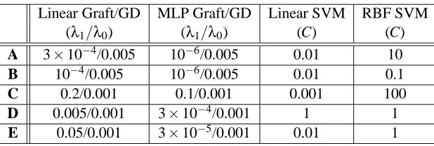
Linear Graft/GD MLP Graft/GD Linear SVM RBF SVM (λ1/λ0) (λ1/λ0) (C) (C) A 3×10⁻⁴/0.005 10−6/0.005 0.01 10 B 10−4/0.005 10−6/0.005 0.01 0.1
C 0.2/0.001 0.1/0.001 0.001 100
D 0.005/0.001 3×10⁻⁴/0.001 1 1 E 0.05/0.001 3×10⁻⁵/0.001 0.01 1
Table 2: Regularization parameters used in experiments for each dataset, chosen using five-fold cross-validation. “GD” stands for Gradient Descent.
4.3 Experimental Details
Each algorithm was applied to each of the datasets. The exception to this was the fully connected MLP (algorithm (d)), which failed to converge for several of the larger datasets. We suspect that this was caused by the large number of weights close to zero in the model, and the discontinuous derivative of the regularizer at this point. For the three synthetic problems the training runs were repeated for ten different random instantiations of the training and test sets, to assess sensitivity to small changes in the dataset.
The regularization parameters used in these experiments were chosen using five-fold cross val-idation on each of the training sets. Algorithms (a) and (c) share the same parameters; as do algo-rithms (b) and (d); and algoalgo-rithms (f), (g) and (h). Note that the grafting algoalgo-rithms, (a) and (b), use bothΩ1andΩ0regularization, requiring parametersλ1andλ0, while the corresponding simple gradient descent algorithms, (c) and (d), use only Ω1 regularization. This is due to the difficulty of incorporatingΩ0 regularization into a standard gradient descent algorithm. The parameters are listed in Table 2.
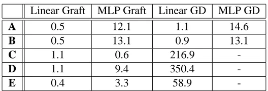
For the Matlab implementations (algorithms (a), (b), (c) and (d)) the training time on each dataset was recorded to see if grafting gave a speedup over simple gradient descent. A direct speed comparison between the SVM algorithms (written in C) and the Matlab implementations was not attempted at this time, due to the inherent efficiency differences between Matlab and C code.
We also recorded the number of features selected (not the same as the number of weights in general), for those algorithms that select a subset of the features (all algorithm except (e) and (f)). In addition, for the three synthetic problems, we can directly calculate a measure of how useful the selected feature subsets are. Recall that in each of these problems there are nrinformative features,
not including redundant duplicates. We can define a feature set saliency measure:
s=ng nr +
ng
nf −
1
where ng is the number of “good” features selected (i.e. informative features, but not including
any duplicate redundant features), and nf is the total number of features selected. The saliency
evaluates to 1 if all nr good features are selected and no others are selected. It evaluates to -1 if
no good features are selected, and it evaluates to approximately zero if all the good features are selected, but only along with many irrelevant or redundant features.
Linear Graft MLP Graft Linear GD MLP GD
A 0.5 12.1 1.1 14.6
B 0.5 13.1 0.9 13.1
C 1.1 0.6 216.9
-D 1.1 9.4 350.4
-E 0.4 3.3 58.9
-Table 3: Timing comparisons for Matlab-implemented algorithms on the five datasets. The entries in the table are the mean number of CPU seconds used by each training algorithm on each dataset. Note that the MLP gradient descent algorithm could not be applied to the larger datasets due to convergence problems.
feature subset saliency should be treated with some suspicion for these two algorithms. Grafting avoids this issue by only adjusting weights that are likely to end up as non-zero.
4.4 Results and Analysis
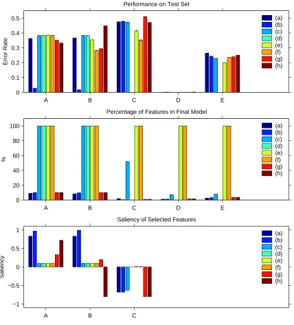
Figure 3 summarizes the test performance and subset selection results of the experiments. Table 3 details the mean run time for the various Matlab algorithms on each dataset.
We will consider the results for each dataset in turn.
Dataset A 90% of the features in this dataset are irrelevant, while each of the others is only weakly relevant by itself. The problem is not linearly separable so the error rate of the linear algorithms (a), (c) and (e) probably couldn’t be much better than the observed 0.36–0.38 level, even with an optimal choice of hyperplane. Curiously enough though, the non-linear SVM algorithm (f) also performed badly, presumably due to the large number of irrelevant features. Adding subset selection to the non-linear SVM made it perform somewhat better — the filter selection method (g) slightly outperforming the wrapper method (h). The winner by a very long way though is the MLP graft algorithm (b). The reasons behind these performance differences can largely be explained by the saliency chart. The gradient test heuristic was able to pick out just the salient features with almost 100% accuracy, and the MLP was flexible enough to fit the non-linear discriminant boundary to a high degree of accuracy. The linear grafting algorithm also picked out good sets of features, but was unable to exploit these due to its inflexible model. The correlation filter method picked the third most salient set of features and came third in terms of performance. It is very likely that at least some of the performance difference between the MLP grafting algorithm and the non-linear SVM, is due to the fact that the MLP network matches the structure of the threshold max problem better than an RBF network.
A B C D E 0
0.1 0.2 0.3 0.4 0.5
Error Rate
Performance on Test Set
(a) (b) (c) (d) (e) (f) (g) (h)
A B C D E
0 20 40 60 80 100
%
Percentage of Features in Final Model
(a) (b) (c) (d) (e) (f) (g) (h)
A B C
−1 −0.5 0 0.5 1
Saliency
Saliency of Selected Features
(a) (b) (c) (d) (e) (f) (g) (h)
filter-based subset selection technique. This is to be expected since this simple filter has no reason not to pick multiple redundant features.
Dataset C With 1000 dimensions and only 100 training points this is a very hard problem. Look-ing at the saliency chart, it is clear that the graftLook-ing algorithms, along with both the wrapper and filter selection methods, pick out very poor subsets of features. The only algorithms to perform much bet-ter than a random classifier are the two SVM algorithms without subset selection, (e) and (f). The non-linear SVM performs best by a significant margin. The problem seems to be that, given enough features and few enough data points, the grafting and other subset selection methods are very likely to find irrelevant features that explain the labels better than the true informative features, merely by chance. They then seize on those features as the most useful. In contrast, the basic SVM, with l2 regularization and no subset selection, has less tendency to focus on just a few features, and so does better.
Dataset D The digit recognition problem turns out to be very easy, with most algorithms misclas-sifying only one member of the test set, out of 1000. The challenge here is to solve the problem quickly and using as few features as possible — many of the features are relatively expensive to compute so this is a real-world challenge. The linear and non-linear grafting algorithms (a) and (b) do an excellent job in this respect, achieving excellent performance using only about 1% of the features. This parsimony also pays off in terms of training time, as the linear grafting algorithm is over 300 times faster than training a full linear model using gradient descent.
Dataset E The arrhythmia problem is quite a hard one. The best algorithm is the linear SVM (e), with an average error rate of around 0.2. All the other algorithms achieve performance figures in the vicinity of 0.25, although the grafting algorithms achieve this error rate using a very small fraction of the available features.
5. Discussion
We finish with some conclusions, and compare grafting to some better-known algorithms.
5.1 Connections with Stagewise Additive Modelling
Both the linear and MLP models considered in this paper are examples of additive models:
E(y|x) =
k
∑
i=1 fi(x)
Hastie et al. (2001, chap. 9) provide an in-depth discussion of this class of models which have a long history in statistics. They also describe a method called additive regression that allows us to fit the above model using backfitting (Friedman and Stuetzle, 1981). Backfitting is a simple iterative procedure whereby the individual functions fi are adjusted one at a time to optimize a chosen loss
As an alternative to using a model with a fixed number of components k, we can incrementally develop such a model using a greedy stagewise algorithm. In this approach, at each time step, we add a new component to the additive model, which is designed to reduce the current loss as much as possible. The previous components are fixed, and only the new function is adjusted. An example of this is matching pursuit, described by Mallat and Zhang (1993). This approach is also discussed at length by Friedman et al. (2000) where they develop a greedy stagewise form of additive logistic regression.
All this looks very similar to the grafting procedure described in this paper, so what is new about grafting? Here are some of the more important differences:
• Grafting is used to build up models out of components that may be combined together in much more complicated ways than simply being added together. In MLP graft, for instance, at each grafting step we consider both adding a new hidden node, and adding an input to an existing node. These options are considered in the same framework, but involve rather differ-ent alterations to the model. In stagewise additive modelling we are usually only concerned with adding another fi to the model at each step.
• At each step, grafting considers many possibilities for altering the current model (typically one for each weight in
F
) and decides between them using the gradient test heuristic. In stagewise additive modelling, we usually only consider one possibility, which is to add (liter-ally) a new function fi, which will be fit to a weighted version of the training set.• After updating the model, stagewise additive modelling typically only adjusts parameters relating to the most recently added fi. Grafting usually adjusts all the free parameters in
the model using a gradient descent engine. This is feasible because our model output is always differentiable with respect to all the model parameters. Additive model practitioners do sometimes use backfitting to fit their models, but this is likely to be less efficient than using a quasi-Newton gradient descent algorithm.
5.2 Connections with Boosting
Boosting (Freund and Schapire, 1996) is one of the most active fields of research in modern machine learning. Boosting, and in particular the AdaBoost algorithm, provides a way of training a sequence of classifiers on some data and then combining them together to form an ensemble classifier that is substantially better than any of its member classifiers.
Boosting can be viewed as a form of stagewise additive modelling (Friedman et al., 2000) that optimizes a logistic regression-like loss function, combined with an l1 regularizer. It works by reweighting the training data at each stage, training a new classifier using a “weak learner”, and forming a composite classifier as a linear combination of the classifiers learned at each stage. The reweighting of the data can be shown to “encourage” a new classifier to be learned that maximally decreases the logistic regression loss (Friedman et al., 2000).
If we consider the variant of grafting mentioned in Section 3.4, where we only update the most recently added weights, and use a linear model withΩ1regularization, then we end up with some-thing that is very much like an extreme version of boosting where the weak learner simply fits a model of the form f(x) =w0+w1xk, choosing a single feature xk to add to the model. The
versions of boosting relax this requirement (Schapire and Singer, 1999) however, so in fact this variant of linear grafting is a simple form of boosting.
The original boosting algorithm mandated an l1regularizer and the logistic regression loss func-tion. However, Mason et al. (2000) have devised a general purpose algorithm called AnyBoost, which, like grafting (and stagewise additive modelling) can work with a variety of loss functions and regularization methods.
5.3 Implications for Regularization
We achieved best performance with the grafting algorithms using both aΩ1and aΩ0regularizer. It has been argued, (e.g., see Tibshirani, 1994), thatΩ1regularization represents a good compromise between the needs of coefficient shrinkage for generalization performance, and the needs of subset selection for pragmatic reasons. However, as discussed in Section 2.1.2, these are really two separate goals and perhaps should be accounted for separately. Our experience is that if we attempted to use onlyΩ1regularization then it was often impossible to find a single value ofλ1that produced good generalization performance without also incorporating many largely irrelevant features. It should be noted, though, that theΩqregularizer with q=1 is the smallest q-value where the regularizer is
convex.
5.4 Other Related Work
Das (2001) describes a technique for using boosting for feature selection. However he does not combine feature selection with model building in the integrated way we have described.
Jebara and Jaakkola (2000) also examine feature selection in a regularized risk minimization context for linear models. They define a prior describing likely values of weights, and choose one that tends to drive a number of weights to zero, in a similar fashion to l1 regularization. In fact l1 regularization can be viewed as being equivalent to a sharply peaked prior for weight values (Tibshirani, 1994).
Weston et al. (2000) describe a gradient descent method that can be used to select a subset of features non-linear for support vector machines. The input features are first weighted using a vector of weights σ. This vector is then optimized using gradient descent, to minimize a bound on the expected leave-one-out error, subject to a l1constraint on the magnitude ofσ. This leads to some of the elements ofσbeing driven to zero.
SVMs are normally associated with l2regularization, but it is possible to formulate them using an l1norm as well. Fung and Mangasarian (2002) describe a gradient descent technique for rapidly optimizing such l1SVMs, which have the property that, as usual, many weights are driven to zero.
References
C.L. Blake and C.J. Merz. UCI repository of machine learning databases. http://www.ics.uci.edu/˜mlearn/MLRepository.html, 1998. University of Califor-nia, Irvine, Dept. of Information and Computer Science.
C. Chang and C. Lin. LIBSVM: A library for support vector machines. Software available at http://www.csie.ntu.edu.tw/˜cjlin/libsvm, 2001.
S. Das. Filters, wrappers and a boosting-based hybrid for feature selection. In Proc. ICML. Morgan Kauffmann, 2001.
Y. Freund and R.E. Schapire. Experiments with a new boosting algorithm. In Machine Learning: Proc. 13th Int. Conf., pages 148–156. Morgan Kaufmann, 1996.
J. Friedman, T. Hastie, and R. Tibshirani. Additive logistic regression: A statistical view of boosting. Annals of Statistics, 28:337–307, 2000.
J. Friedman and W. Stuetzle. Projection pursuit regression. Journal of the American Statistical Association, 76:817–823, 1981.
G. Fung and O.L. Mangasarian. A feature selection Newton method for support vector machine classification. Technical Report 02-03, Data Mining Institute, Dept. of Computer Sciences, Uni-versity of Wisconsin: Madison, Sept 2002.
F. Girosi, M. Jones, and T. Poggio. Regularization theory and neural networks architectures. Neural Computation, 7:219–269, 1995.
T. Hastie, R. Tibshirani, and J. Friedman. The Elements of Statistical Learning. Springer, 2001.
A.E. Hoerl and R. Kennard. Ridge regression: Biased estimation for nonorthogonal problems. Technometrics, 12:55–67, 1970.
T. Jebara and T. Jaakkola. Feature selection and dualities in maximum entropy discrimination. In Proc. Int. Conf. on Uncertainity in Artificial Intelligence, 2000.
K. Kira and L. Rendell. A practical approach to feature selection. In D. Sleeman and P. Edwards, editors, Proc. Int. Conf. on Machine Learning, pages 249–256. Morgan Kaufmann, 1992.
R. Kohavi and G.H. John. Wrappers for feature subset selection. Artificial Intelligence, 97:273–324, 1997.
S. Mallat and Z. Zhang. Matching pursuit with time-frequency dictionaries. IEEE Transactions on Signal Processing, 41(12):3397–3415, 1993.
L. Mason, J. Baxter, P.L. Bartlett, and M. Frean. Functional gradient techniques for combining hypotheses. In A.J. Smola, P.L Bartlett, B. Sc¨olkopf, and D. Schuurmans, editors, Advances in Large Margin Classifiers, pages 221–246. MIT Press, 2000.
J.A. Nelder and R. Mead. A simplex method for function minimization. Computer Journal, 7: 308–313, 1965.
W.H. Press, S.A. Teukolsky, W.T. Vetterling, and B.P. Flannery. Numerical Recipes in C. Cambridge University Press, 2nd edition, 1992.
B. Sch¨olkopf and A. Smola. Learning with Kernels. MIT Press, Cambridge, MA, 2002.
A.J. Smola, P.J. Bartlett, B. Sch¨olkopf, and D. Schuurmans, editors. Advances in Large Margin Classifiers. MIT Press, 2000.
R. Tibshirani. Regression shrinkage and selection via the lasso. Technical report, Dept. of Statistics, University of Toronto, 1994.