Spectral Ranking using Seriation
Fajwel Fogel [email protected]
C.M.A.P. ´
Ecole Polytechnique Palaiseau, France.
Alexandre d’Aspremont [email protected]
CNRS & DI, UMR 8548 ´
Ecole Normale Sup´erieure Paris, France.
Milan Vojnovic [email protected]
Microsoft Research Cambridge, U.K.
Editor:Aapo Hyvarinen
Abstract
We describe a seriation algorithm for ranking a set of items given pairwise comparisons between these items. Intuitively, the algorithm assigns similar rankings to items that com-pare similarly with all others. It does so by constructing a similarity matrix from pairwise comparisons, using seriation methods to reorder this matrix and construct a ranking. We first show that this spectral seriation algorithm recovers the true ranking when all pairwise comparisons are observed and consistent with a total order. We then show that ranking reconstruction is still exact when some pairwise comparisons are corrupted or missing, and that seriation based spectral ranking is more robust to noise than classical scoring meth-ods. Finally, we bound the ranking error when only a random subset of the comparions are observed. An additional benefit of the seriation formulation is that it allows us to solve semi-supervised ranking problems. Experiments on both synthetic and real datasets demonstrate that seriation based spectral ranking achieves competitive and in some cases superior performance compared to classical ranking methods.
Keywords: Ranking, seriation, spectral methods
1. Introduction
We study the problem of ranking a set ofnitems given pairwise comparisons between these items1. The problem of aggregating binary relations has been formulated more than two centuries ago, in the context of emerging social sciences and voting theories (de Borda, 1781; de Condorcet, 1785). The setting we study here goes back at least to (Zermelo, 1929; Kendall and Smith, 1940) and seeks to reconstruct a ranking of items from pairwise comparisons reflecting a total ordering. In this case, the directed graph of all pairwise comparisons, where every pair of vertices is connected by exactly one of two possible directed edges, is usually called atournamentgraph in the theoretical computer science literature or a “round
robin” in sports, where every player plays every other player once and each preference marks victory or defeat. The motivation for this formulation often stems from the fact that in many applications, e.g. music, images, and movies, preferences are easier to express in relative terms (e.g. ais better thanb) rather than absolute ones (e.g. a should be ranked fourth, and bseventh). In practice, the information about pairwise comparisons is usually
incomplete, especially in the case of a large set of items, and the data may also be noisy, that is some pairwise comparisons could be incorrectly measured and inconsistent with a total order.
ranking are derived using classical algorithms, e.g., Borda Count, Bradley-Terry-Model maximum likelihood estimation, least squares, odd-ratios (Saaty, 2003).
Here, we show that the ranking problem is directly related to another classical ordering problem, namelyseriation. Given a similarity matrix between a set ofnitems and assuming that the items can be ordered along a chain (path) such that the similarity between items decreases with their distance within this chain (i.e. a total order exists), the seriation problem seeks to reconstruct the underlying linear ordering based on unsorted, possibly noisy, pairwise similarity information. Atkins et al. (1998) produced a spectral algorithm that exactly solves the seriation problem in the noiseless case, by showing that for similarity matrices computed from serial variables, the ordering of the eigenvector corresponding to the second smallest eigenvalue of the Laplacian matrix (a.k.a. the Fiedler vector) matches that of the variables. In practice, this means that performing spectral ordering on the similarity matrix exactly reconstructs the correct ordering provided items are organized in a chain.
We adapt these results to ranking to produce a very efficient spectral ranking algorithm with provable recovery and robustness guarantees. Furthermore, the seriation formulation allows us to handle semi-supervised ranking problems. Fogel et al. (2013) show that seriation is equivalent to the 2-SUM problem and study convex relaxations to seriation in a semi-supervised setting, where additional structural constraints are imposed on the solution. Several authors (Blum et al., 2000; Feige and Lee, 2007) have also focused on the directly related Minimum Linear Arrangement (MLA) problem, for which excellent approximation guarantees exist in the noisy case, albeit with very high polynomial complexity.
The main contributions of this paper can be summarized as follows. We link seriation and ranking by showing how to construct a consistent similarity matrix based on consistent pairwise comparisons. We then recover the true ranking by applying the spectral seriation algorithm in (Atkins et al., 1998) to this similarity matrix (we call this method SerialRank in what follows). In the noisy case, we then show that spectral seriation can perfectly recover the true ranking even when some of the pairwise comparisons are either corrupted or missing, provided that the pattern of errors is somewhat unstructured. We show in particular that, in a regime where a high proportion of comparisons are observed, some incorrectly, the spectral solution is more robust to noise than classical scoring based methods. On the other hand, when only few comparisons are observed, we show that for Erd¨os-R´enyi graphs, i.e., when pairwise comparisons are observed independently with a given probability, Ω(nlog4n) comparisons suffice for`2 consistency of the Fiedler vector and hence`2 consistency of the retreived ranking w.h.p. On the other hand we need Ω(n3/2log4n) comparisons to retrieve a ranking whose local perturbations are bounded in`∞norm. Since for Erd¨os-R´enyi graphs the induced graph of comparisons is connected with high probability only when the total number of pairs sampled scales as Ω(nlogn) (aka the coupon collector effect), we need at least that many comparisons in order to retrieve a ranking, therefore the `2 consistency result can be seen as optimal up to a polylogarithmic factor. Finally, we use the seriation results in (Fogel et al., 2013) to produce semi-supervised ranking solutions.
In Section 4 we then show that this spectral solution remains exact in a noisy regime where a random subset of comparisons is corrupted. In Section 5 we analyze ranking perturbation results when only few comparisons are given following an Erd¨os-R´enyi graph. Finally, in Section 6 we illustrate our results on both synthetic and real datasets, and compare ranking performance with classical MLE, spectral and scoring based approaches.
2. Seriation, Similarities & Ranking
In this section we first introduce the seriation problem, i.e. reordering items based on pairwise similarities. We then show how to write the problem of ranking given pairwise comparisons as a seriation problem.
2.1 The Seriation Problem
The seriation problem seeks to reordernitems given a similarity matrix between these items, such that the more similar two items are, the closer they should be. This is equivalent to supposing that items can be placed on a chain where the similarity between two items decreases with the distance between these items in the chain. We formalize this below, following (Atkins et al., 1998).
Definition 1 We say that a matrix A ∈ Sn is an R-matrix (or Robinson matrix) if and only if it is symmetric and Ai,j ≤ Ai,j+1 and Ai+1,j ≤ Ai,j in the lower triangle, where 1≤j < i≤n.
Another way to formulate R-matrix conditions is to imposeAij ≥Akl if|i−j| ≤ |k−l| off-diagonal, i.e. the coefficients of A decrease as we move away from the diagonal. We also introduce a definition for strict R-matrices A, whose rows and columns cannot be permuted without breaking the R-matrix monotonicity conditions. We callreverse identity
permutation the permutation that puts rows and columns 1,2, . . . , nof a matrixAin reverse order n, n−1, . . . ,1.
Definition 2 An R-matrix A∈Sn is called strict-R if and only if the identity and reverse identity permutations of A are the only permutations reorderingA as an R-matrix.
Any R-matrix with only strict R-constraints is a strict R-matrix. Following (Atkins et al., 1998), we will say that A is pre-R if there is a permutation matrix Π such that ΠAΠT is an R-matrix. Given a pre-R matrixA, the seriation problem consists in finding a permutation Π such that ΠAΠT is an R-matrix. Note that there might be several solutions to this problem. In particular, if a permutation Π is a solution, then the reverse permutation is also a solution. When only two permutations of A produce R-matrices,A will be called
pre-strict-R.
2.2 Constructing Similarity Matrices from Pairwise Comparisons
similarity between two items decreases with the distance between their ranks. We will then be able to use the spectral seriation algorithm by (Atkins et al., 1998) described in Section 3 to reconstruct the true ranking from a disordered similarity matrix.
We first show how to compute a pairwise similarity from pairwise comparisons between items by counting the number of matching comparisons. Another formulation allows us to handle the generalized linear model. These two examples are only two particular instances of a broader class of ranking algorithms derived here. Any method which produces R-matrices from pairwise preferences yields a valid ranking algorithm.
2.2.1 Similarities from Pairwise Comparisons
Suppose we are given a matrix of pairwise comparisonsC∈ {−1,0,1}n×nsuch that C i,j =
−Cj,i for everyi6=j and
Ci,j =
1 ifiis ranked higher than j
0 ifiand j are not compared or in a draw −1 ifj is ranked higher than i
(1)
setting Ci,i = 1 for all i∈ {1, . . . , n}. We define the pairwise similarity matrixSmatch as
Si,jmatch= n X
k=1
1 +Ci,kCj,k 2
. (2)
Since Ci,kCj,k = 1, if Ci,k and Cj,k have matching signs, and Ci,kCj,k = −1 if they have opposite signs, Si,jmatch counts the number of matching comparisons between i and j with other reference items k. If ior j is not compared withk, then Ci,kCj,k = 0 and the term (1 +Ci,kCj,k)/2 has an neutral effect on the similarity of 1/2. Note that we also have
Smatch= 1 2 n11
T +CCT
. (3)
The intuition behind the similarity Smatch is easy to understand in a tournament setting: players that beat the same players and are beaten by the same players should have a similar ranking.
The next result shows that when all comparisons are given and consistent with the identity ranking, then the similarity matrix Smatch is a strict R-matrix. Without loss of generality, we assume that items are ranked in increasing order of their indices. In the general case, we can simply replace the strict-R property by thepre-strict-R property.
Proposition 3 Given all pairwise comparisons between items ranked according to the iden-tity permutation (with no ties), the similarity matrix Smatch constructed in (2) is a strict R-matrix and
Si,jmatch=n− |i−j| (4)
ProofSince items are ranked as 1,2, . . . , nwith no ties and all comparisons given,Ci,j =−1 ifi < j andCi,j = 1 otherwise. Therefore we obtain from definition (2)
Si,jmatch =
min(i,j)−1 X
k=1
1 + 1 2
+
max(i,j)−1 X
k=min(i,j)
1−1 2
+
n X
k=max(i,j)
1 + 1 2
= n−(max(i, j)−min(i, j))
= n− |i−j|
This means in particular that Smatch is strictly positive and its coefficients are strictly de-creasing when moving away from the diagonal, henceSmatch is a strict R-matrix.
2.2.2 Similarities in the Generalized Linear Model
Suppose that paired comparisons are generated according to a generalized linear model (GLM), i.e., we assume that the outcomes of paired comparisons are independent and for any pair of distinct items, itemiis observed ranked higher than itemj with probability
Pi,j =H(νi−νj) (5)
where ν ∈ Rn is a vector of skill parameters and H : R → [0,1] is a function that is increasing on R and such that H(−x) = 1−H(x) for all x ∈ R, and limx→−∞H(x) = 0 and limx→∞H(x) = 1. A well known special instance of the generalized linear model is the Bradley-Terry-Luce model for which H(x) = 1/(1 +e−x), forx∈R.
Let mi,j be the number of times items i and j were compared, Ci,js ∈ {−1,1} be the outcome of comparisonsand Qbe the matrix of corresponding sample probabilities, i.e. if mi,j >0 we have
Qi,j = 1 mi,j
mi,j
X
s=1
Ci,js + 1 2
andQi,j = 1/2 in casemi,j = 0. We define the similarity matrixSglm from the observations Qas
Si,jglm = n X
k=1
1{mi,kmj,k>0}(1− |Qi,k−Qj,k|) +
1{mi,kmj,k=0}
2 . (6)
Since the comparison observations are independent we have that Qi,j converges toPi,j as mi,j goes to infinity and the central limit theorem implies thatSi,jglmconverges to a Gaussian variable with mean
n X
k=1
(1− |Pi,k−Pj,k|).
The result below shows that this limit similarity matrix is a strict R-matrix when items are properly ordered.
ProofWithout loss of generality, we suppose the true order is 1,2, . . . , n, withν(1)> . . . > ν(n). For any i, j, k such that i > j, using the GLM assumption (i) we get
Pi,k =H(ν(i)−ν(k))< H(ν(j)−ν(k)) =Pj,k.
Since empirical probabilitiesQi,j converge toPi,j, when the number of observations is large enough, we also have Qi,k < Qj,k for any i, j, k such that i > j (we focus w.l.o.g. on the lower triangle), and we can therefore remove the absolute value in the expression of Si,jglm fori > j. Hence for any i > j we have
Si+1,jglm −Si,jglm = −
n X
k=1
|Qi+1,k−Qj,k|+ n X
k=1
|Qi,k −Qj,k|
= n X
k=1
(Qi+1,k−Qj,k)−(Qi,k −Qj,k)
= n X
k=1
Qi+1,k−Qi,k <0.
Similarly for any i > j,Si,jglm−1−Si,jglm <0, so Sglm is a strict R-matrix.
Notice that we recover the original definition ofSmatch in the case of binary comparisons, though it does not fit in the Generalized Linear Model. Note also that these definitions can be directly extended to the setting where multiple comparisons are available for each pair and aggregated in comparisons that take fractional values (e.g., a tournament setting where participants play several times against each other).
3. Spectral Algorithms
We first recall how spectral ordering can be used to recover the true ordering in seriation problems. We then apply this method to the ranking problem.
3.1 Spectral Seriation Algorithm
We use the spectral computation method originally introduced in (Atkins et al., 1998) to solve the seriation problem based on the similarity matrices defined in the previous section. We first recall the definition of the Fiedler vector (which is shown to be unique in our setting in Lemma 7).
Definition 5 The Fiedler value of a symmetric, nonnegative and irreducible matrix A is the smallest non-zero eigenvalue of its Laplacian matrix LA =diag(A1)−A. The corre-sponding eigenvector is called Fiedler vector and is the optimal solution to min{yTLAy : y∈Rn, yT1= 0,kyk
2 = 1}.
Proposition 6 (Atkins et al., 1998, Th. 3.3) Let A ∈ Sn be an irreducible pre-R-matrix with a simple Fiedler value and a Fiedler vector v with no repeated values. Let Π1 ∈ P (respectively, Π2) be the permutation such that the permuted Fiedler vector Π1v is strictly increasing (decreasing). Then Π1AΠT1 and Π2AΠT2 are R-matrices, and no other permuta-tions of A produce R-matrices.
The next technical lemmas extend the results in Atkins et al. (1998) to strict R-matrices and will be used to prove Theorem 10 in next section. The first one shows that without loss of generality, the Fiedler value is simple.
Lemma 7 If A is an irreducible R-matrix, up to a uniform shift of its coefficients, A has a simple Fiedler value and a monotonic Fiedler vector.
ProofWe use (Atkins et al., 1998, Th. 4.6) which states that ifAis an irreducible R-matrix with An,1 = 0, then the Fiedler value of A is a simple eigenvalue. Since A is an R-matrix, An,1is among its minimal elements. Subtracting it fromAdoes not affect the nonnegativity of A and we can apply (Atkins et al., 1998, Th. 4.6). Monotonicity of the Fiedler vector then follows from (Atkins et al., 1998, Th. 3.2).
The next lemma shows that the Fiedler vector is strictly monotonic if A is a strict R-matrix.
Lemma 8 Let A ∈ Sn be an irreducible R-matrix. Suppose there are no distinct indices r < s such that for any k 6∈[r, s], Ar,k= Ar+1,k =. . .=As,k, then, up to a uniform shift, the Fiedler value of A is simple and its Fiedler vector is strictly monotonic.
Proof By Lemma 7, the Fiedler value of A is simple (up to a uniform shift of A). Let x be the corresponding Fiedler vector of A, x is monotonic by Lemma 7. Suppose [r, s] is a nontrivial maximal interval such that xr = xr+1 = . . . = xs, then by (Atkins et al., 1998, lemma 4.3), for anyk6∈[r, s], Ar,k=Ar+1,k =. . .=As,k, which contradicts the initial assumption. Thereforex is strictly monotonic.
In fact, we only need a small portion of the R-constraints to be strict for the previous lemma to hold. We now show that the main assumption onA in Lemma 8 is equivalent to A being strict-R.
Lemma 9 An irreducible R-matrix A∈Sn is strictlyR if and only if there are no distinct indicesr < s such that for any k6∈[r, s], Ar,k=Ar+1,k =. . .=As,k.
Algorithm 1 (SerialRank)
Input: A set of pairwise comparisons Ci,j ∈ {−1,0,1} or [−1,1].
1: Compute a similarity matrixS as in§2.2
2: Compute the Laplacian matrix
LS=diag(S1)−S (SerialRank)
3: Compute the Fiedler vector ofS.
Output: A ranking induced by sorting the Fiedler vector ofS (choose either increasing or decreasing order to minimize the number of upsets).
k 6∈ [r, s], Ar,k =Ar+1,k =. . . = As,k. Therefore at least four different permutations of A produce R-matrices, which means thatA is not strictly R.
3.2 SerialRank: a Spectral Ranking Algorithm
In Section 2, we showed that similarities Smatch and Sglm are pre-strict-R when all com-parisons are available and consistent with an underlying ranking of items. We now use the spectral seriation method in (Atkins et al., 1998) to reorder these matrices and pro-duce a ranking. Spectral ordering requires computing an extremal eigenvector, at a cost of O(n2logn) flops (Kuczynski and Wozniakowski, 1992). We call this algorithm SerialRank and prove the following result.
Theorem 10 Given all pairwise comparisons for a set of totally ordered items and assum-ing there are no ties between items, algorithm SerialRank, i.e., sortassum-ing the Fiedler vector of the matrix Smatch defined in (3), recovers the true ranking of items.
Proof From Proposition 3, under assumptions of the proposition Smatch is a pre-strict R-matrix. Now combining the definition of strict-R matrices in Lemma 9 with Lemma 8, we deduce that Fiedler value of Smatch is simple and its Fiedler vector has no repeated values. Hence by Proposition 6, only the two permutations that sort the Fiedler vector in increasing and decreasing order produce strict R-matrices and are candidate rankings (by Proposition 3 Smatch is a strict R-matrix when ordered according to the true ranking). Finally we can choose between the two candidate rankings (increasing and decreasing) by picking the one with the least upsets.
4. Exact Recovery with Corrupted and Missing Comparisons
In this section we study the robustness of SerialRank using Smatch with respect to noisy and missing pairwise comparisons. We will see that noisy comparisons cause ranking ambi-guities for the point score method and that such ambiambi-guities are to be lifted by the spectral ranking algorithm. We show in particular that the SerialRank algorithm recovers the exact ranking when the pattern of errors is random and errors are not too numerous. We first study the impact of one corrupted comparison on SerialRank, then extend the result to multiple corrupted comparisons. A similar analysis is provided for missing comparisons as Corollary 27. in the Appendix. Finally, Proposition 14 provides an estimate of the number of randomly corrupted entries that can be tolerated for perfect recovery of the true ranking. We begin by recalling the definition of thepoint score of an item.
Definition 11 Thepoint score wi of an itemi, also known as point-difference, orrow-sum
is defined as wi =Pn
k=1Ck,i, which corresponds to the number of wins minus the number of losses in a tournament setting.
In the following we will denote byw the point score vector.
Proposition 12 Given all pairwise comparisons Cs,t ∈ {−1,1} between items ranked ac-cording to their indices, suppose the sign of one comparison Ci,j (and its counterpart Cj,i) is switched, with i < j. If j−i >2 then Smatch defined in (3) remains strict-R, whereas the point score vector w has ties between items iand i+ 1 and itemsj and j−1.
Proof We give some intuition for the result in Figure 1. We write the true score and comparison matrixwandC, while the observations are written ˆwand ˆC respectively. This means in particular that ˆCi,j =−Ci,j = 1 and ˆCj,i=−Cj,i=−1. To simplify notations we denote by S the similarity matrix Smatch (respectively ˆS when the similarity is computed from observations). We first study the impact of a corrupted comparison Ci,j fori < j on the point score vector ˆw. We have
ˆ wi =
n X
k=1 ˆ Ck,i=
n X
k=1
Ck,i+ ˆCj,i−Cj,i =wi−2 =wi+1,
similarly ˆwj =wj−1, whereas ˆwk =wkfork6=i, j. Hence, the incorrect comparison induces two ties in the point score vectorw. Now we show that the similarity matrix defined in (3) breaks these ties, by showing that it is a strict R-matrix. Writing ˆS in terms of S, we get for any t6=i, j
[ ˆCCˆT]i,t= X
k6=j
ˆ Ci,kCt,kˆ
+ ˆCi,jCt,jˆ =X k6=j
(Ci,kCt,k) + ˆCi,jCt,j =
[CCT]i,t−2 ift < j
CCT
i,t+ 2 ift > j. Thus we obtain
ˆ Si,t =
Si,t−1 ift < j Si,t+ 1 ift > j,
(remember there is a factor 1/2 in the definition ofS). Similarly we get for anyt6=i, j
ˆ Sj,t=
Finally, for the single corrupted index pair (i, j), we get
ˆ Si,j =
1 2
n+ X
k6=i,j
ˆ Ci,kCˆj,k
+ ˆCi,iCˆj,i+ ˆCi,jCˆj,j
=Si,j−1 + 1 =Si,j.
The diagonal of S is not impacted since [ ˆCCˆT]i,i = Pnk=1
ˆ Ci,kCˆi,k
= n. For all other
coefficients (s, t) such that s, t6= i, j, we also have ˆSs,t =Ss,t, which means that all rows or columns outside of i, j are left unchanged. We first observe that these last equations, together with our assumption that j−i >2 and the fact that the elements of the exact S in (4) differ by at least one, imply that
ˆ
Ss,t≤Ss+1,tˆ and Ss,t+1ˆ ≤Ss,t,ˆ fors < t
so ˆS remains an R-matrix. Note that this result remains true even when j−i = 2, but we need some strict inequalities to show uniqueness of the retrieved order. Indeed, because j−i >2 all theseR constraints are strict except between elements of rowsiand i+ 1, and rows j−1 andj (and similarly for columns). These ties can be broken using the fact that
ˆ
Si,j−1=Si,j−1−1< Si+1,j−1−1 = ˆSi+1,j−1−1<Sˆi+1,j−1
which means that ˆSis still a strict R-matrix (see Figure 1) sincej−1> i+1 by assumption.
We now extend this result to multiple errors.
Proposition 13 Given all pairwise comparisons Cs,t ∈ {−1,1} between items ranked ac-cording to their indices, suppose the signs of m comparisons indexed (i1, j1), . . . ,(im, jm) are switched. If the following condition (7) holds true,
|s−t|>2, for all s, t∈ {i1, . . . , im, j1, . . . , jm} withs6=t, (7) thenSmatch defined in (3)remains strict-R, whereas the point score vectorw has 2m ties. Proof We write the true score and comparison matrix w and C, while the observations are written ˆw and ˆC respectively, and without loss of generality we suppose il < jl. This implies that ˆCil,jl =−Cil,jl = 1 and ˆCjl,il=−Cjl,il =−1 for alllin{1, . . . , m}. To simplify
notations, we denote by S the similarity matrixSmatch (respectively ˆS when the similarity is computed from observations).
As in the proof of Proposition 12, corrupted comparisons indexed (il, jl) induce shifts of ±1 on columns and rows il and jl of the similarity matrix Smatch, while Simatchl,jl values
remain the same. Since there are several corrupted comparisons, we also need to check the values of ˆS at the intersections of rows and columns with indices of corrupted comparisons. Formally, for any (i, j)∈ {(i1, j1), . . . (im, jm)} and t6∈ {i1, . . . , im, j1, . . . , jm}
ˆ Si,t =
Similarly for t6∈ {i1, . . . , im, j1, . . . , jm} ˆ Sj,t=
Sj,t−1 ift < i Sj,t+ 1 ift > i.
Let (s, s0) and (t, t0)∈ {(i1, j1), . . . (im, jm)}, we have ˆ
Ss,t = 12
n+P k6=s0,t0
ˆ Cs,kCˆt,k
+ ˆCs,s0Cˆt,s0+ ˆCs,t0Cˆt,t0
= 12
n+P
k6=s0,t0(Cs,kCt,k)−Cs,s0Ct,s0 −Cs,t0Ct,t0
Without loss of generality we suppose s < t, and since s < s0 and t < t0, we obtain
ˆ Ss,t=
Ss,t ift > s0 Ss,t+ 2 ift < s0.
Similar results apply for other intersections of rows and columns with indices of corrupted comparisons (i.e., shifts of 0, +2, or −2). For all other coefficients (s, t) such that s, t 6∈ {i1, . . . , im, j1, . . . , jm}, we have ˆSs,t = Ss,t. We first observe that these last equations, together with our assumption thatjl−il>2, mean that
ˆ
Ss,t ≤Ss+1,tˆ and Ss,t+1ˆ ≤Ss,t,ˆ for any s < t
so ˆS remains an R-matrix. Moreover, since jl−il > 2 all these R constraints are strict except between elements of rowsil andil+ 1, and rowsjl−1 andjl (similar for columns). These ties can be broken using the fact that fork=jl−1
ˆ
Sil,k=Sil,k−1< Sil+1,k−1 = ˆSil+1,k−1<Siˆl+1,k
which means that ˆS is still a strict R-matrix sincek=jl−1> il+ 1. Moreover, using the same argument as in the proof of Proposition 12, corrupted comparisons induces 2m ties in the point score vectorw.
For the case of one corrupted comparison, note that the separation condition on the pair of items (i, j) is necessary. When the comparison Ci,j between two adjacent items is cor-rupted, no ranking method can break the resulting tie. For the case of arbitrary number of corrupted comparisons, condition (7) is a sufficient condition only. We study exact ranking recovery conditions with missing comparisons in the Appendix, using similar arguments. We now estimate the number of randomly corrupted entries that can be tolerated while maintaining exact recovery of the true ranking.
ProofLetP be the set of all distinct pairs of items from the set{1,2, . . . , n}. LetX be the set of all admissible sets of pairs of items, i.e. containing eachX ⊆ P such thatX satisfies condition (7). We consider the case ofm ≥1 distinct pairs of items sampled from the set P uniformly at random without replacement. LetXi denote the set of sampled pairs given thatipairs are sampled. We seek to boundp(n, m) =Prob(Xm∈ X). Given a set of pairs X∈ X, letT(X) be the set of non-admissible pairs, i.e. containing (i, j)∈ P \Xsuch that X∪(i, j)∈ X/ . We have
Prob(Xm∈ X) =
X
x∈X:|x|=m−1
1− |T(x)| |P| −(m−1)
Prob(Xm−1 =x). (8)
Note that every selected pair fromP contributes at most 15nnon-admissible pairs. Indeed, given a selected pair (i, j), a non-admissible pair (s, t) should respect one of the following conditions |s−i| ≤2, |s−j| ≤ 2,|t−i| ≤2, |t−j| ≤ 2 or|s−t| ≤2. Given any item s, there are 15 possible choice of tto output a non-admissible pair (s, t), resulting in at most 15n non-admissible pairs for the selected pair (i, j).
Hence, for every x∈ X we have
|T(x)| ≤15n|x|.
Combining this with (8) and the fact that|P|= n2
, we have
Prob(Xm ∈ X)≥ 1− n 15n
2
−(m−1)(m−1) !
Prob(Xm−1 ∈ X).
From this it follows
p(n, m) ≥
m−1 Y
i=1
1− n 15n
2
−(i−1)i !
≥
m−1 Y
i=1
1− i
a(n, m)
where
a(n, m) = n 2
−(m−1)
15n .
Notice that when m=o(n) we have1− i a(n,m)
∼exp(−30i/n) and
m−1 Y
i=1
1− i
a(n, m)
∼
m−1 Y
i=1
exp(−30i/n)∼exp
−15m
2 n
for largen.
5. Spectral Perturbation Analysis
In this section we analyze how SerialRank performs when only a small fraction of pairwise comparisons are given. We show that for Erd¨os-R´enyi graphs, i.e., when pairwise compar-isons are observed independently with a given probability, Ω(nlog4n) comparisons suffice for `2 consistency of the Fiedler vector and hence `2 consistency of the retreived ranking w.h.p. On the other hand we need Ω(n3/2log4n) comparisons to retrieve a ranking whose local perturbations are bounded in`∞norm. Since Erd¨os-R´enyi graphs are connected with high probability only when the total number of pairs sampled scales as Ω(nlogn), we need at least that many comparisons in order to retrieve a ranking, therefore the `2 consistency result can be seen as optimal up to a polylogarithmic factor.
Our bounds are mostly related to the work of (Wauthier et al., 2013). In its simplified version (Theorem 4.2 Wauthier et al., 2013) shows that when ranking items according to their point score, for any precision parameterµ∈(0,1), sampling independently with fixed probability Ωnlogµ2n
comparisons guarantees that the maximum displacement between the retrieved ranking and the true ranking, i.e., the `∞ distance to the true ranking, is bounded by µnwith high probability fornlarge enough.
Sample complexity bounds have also been studied for the Rank Centrality algorithm (Dwork et al., 2001; Negahban et al., 2012). In their analysis, (Negahban et al., 2012) suppose that some pairs are sampled independently with fixed probability, and then k comparisons are generated for each sampled pair, under a Bradley-Terry-Luce model (BTL). When ranking items according to the stationary distribution of a transition matrix estimated from comparisons, sampling Ω(n·polylog(n)) pairs are enough to bound the relative`2 norm perturbation of the stationary distribution. However, as pointed out by (Wauthier et al., 2013), repeated measurements are not practical, e.g., if comparisons are derived from the outcomes of sports games or the purchasing behavior of a customer (a customer typically wants to purchase a product only once). Moreover, (Negahban et al., 2012) do not provide bounds on the relative`∞ norm perturbation of the ranking.
We also refer the reader to the recent work of Rajkumar and Agarwal (2014), who provide a survey of sample complexity bounds for Rank Centrality, maximum likelihood estimation, least-square ranking and an SVM based ranking, under a more flexible sampling model. However, those bounds only give the sampling complexity for exact recovery of ranking, which is usually prohibitive when nis large, and are more difficult to interpret.
Finally, we refer the interested reader to (Huang et al., 2008; Shamir and Tishby, 2011) for sampling complexity bounds in the context of spectral clustering.
Limitations. We emphasize that sampling models based on Erd¨os-R´enyi graphs are not the most realistic, though they have been studied widely in the literature (see for instance Feige et al., 1994; Braverman and Mossel, 2008; Wauthier et al., 2013). Indeed, pairs are not likely to be sampled independently. For instance, when ranking movies, popular movies in the top ranks are more likely to be compared. Corrupted comparisons are also more likely between items that have close rankings. We hope to extend our perturbation analysis to more general models in future work.
for the analysis of SerialRank, since numerical experiments suggest that it is the setting for which SerialRank provides the best results compared to other methods. Note that in prac-tice, we can easily get rid of this limitation (see Section 2.2.2 and 6). We refer the reader to numerical experiments in Section 6, as well as a recent paper by Cucuringu (2015), which introduces another ranking algorithm called SyncRank, and provides extensive numerical experiments on state-of-the-art ranking algorithms, including SerialRank.
Choice of Laplacian: normalized vs. unnormalized. In the spectral clustering literature, several constructions for the Laplacian operators are suggested, namely the un-normalized Laplacian (used in SerialRank), the symmetric un-normalized Laplacian, and the non-symmetric normalized Laplacian. Von Luxburg et al. (2008) show stronger consistency results for spectral clustering by using the non-symmetric normalized Laplacian. Here, we show that the Fiedler vector of the normalized Laplacian is an affine function of the rank-ing, hence sorting the Fiedler vector still guarantees exact recovery of the rankrank-ing, when all comparisons are observed and consistent with a global ranking. In contrast, we only get an asymptotic expression for the unnormalized Laplacian (cf. section A). This motivated us to provide an analysis of SerialRank robustness based on the normalized Laplacian, though in practice the use of the unnormalized Laplacian is valid and seems to give better results (cf.Figures 2 and 5).
Notations. Throughout this section, we only focus on the similarity Smatch in (3) and write it S to simplify notations. W.l.o.g. we assume in the following that the true ranking is the identity, hence S is an R-matrix. We write k · k2 the operator norm of a matrix, which corresponds to the maximal absolute eigenvalue for symmetric matrices. k · kF denotes the Frobenius norm. We refer to the eigenvalues of the Laplacian asλi, with λ1 = 0 ≤ λ2 ≤ . . . ≤ λn. For any quantity x, we denote by ˜x its perturbed analogue. We define the residual matrixR = ˜S−S and write f the normalized Fiedler vector of the Laplacian matrix LS. We define the degree matrix DS = diag(D1) the diagonal matrix whose elements are the row-sums of matrix S. Whenever we use the abreviation w.h.p., this means that the inequality is true with probability greater than 1−2/n. Finally, we will use c > 0 for absolute constants, whose values are allowed to vary from one equation to another.
We assume that our information on preferences is both incomplete and corrupted. Specifically, pairwise comparisons are independently sampled with probability q and these sampled comparisons are consistent with the underlying total ranking with probability p. Let us define ˜C=B◦Cthe matrix of observed comparisons, whereCis the true comparison matrix defined in (1),◦is the Hadamard product andB is a symmetric matrix with entries
Bi,j =
0 with probability 1−q 1 with probability qp
−1 with probability q(1−p).
In order to obtain an unbiased estimator of the comparison matrix defined in (1), we normalize ˜C by its mean valueq(2p−1) and redefine ˜S as
˜
S= 1
q2(2p−1)2C˜C˜
T +n11T.
5.1 Results
We now state our main results. The first one bounds`2 perturbations of the Fiedler vector f with both missing and corrupted comparisons. Note thatf and ˜f are normalized.
Theorem 21 For every µ∈(0,1) and nlarge enough, if q > µ2(2plog−41)n4n, then
kf˜−fk2≤c√µ logn
with probability at least 1−2/n, where c >0 is an absolute constant.
As n goes to infinity the perturbation of the Fiedler vector goes to zero, and we can retrieve the “true” ranking by reordering the Fiedler vector. Hence this bounds provides`2 consistency of the ranking, with an optimal sampling complexity (up to a polylogarithmic factor).
The second result bounds local perturbations of the ranking with π referring to the “true” ranking and ˜π to the ranking retrieved by SerialRank.
Theorem 24 For every µ∈(0,1) and nlarge enough, if q > µ2(2plog−41)n4√n, then
kπ˜−πk∞≤cµn
with probability at least 1−2/n, where c >0 is an absolute constant.
This bound quantifies the maximum displacement of any item’s ranking. µ can be seen a “precision” parameter. For instance, if we set µ= 0.1, Theorem 24 means that we can expect the maximum displacement of any item’s ranking to be less than 0.1·n when observingc2·100·n√n·log4ncomparisons (with p= 1).
We conjecture Theorem 24 still holds true if the condition q >log4n/µ2(2p−1)4√nis replaced by the weaker conditionq >log4n/µ2(2p−1)4n.
5.2 Sketch of the proof.
The proof of these results relies on classical perturbation arguments and is structured as follows.
• Step 1: Bound kD˜S −DSk2, kS˜−Sk2 with high probability using concentration inequalities on quadratic forms of Bernoulli variables and results from (Achlioptas and McSherry, 2007).
• Step 2. Show that the normalized LaplacianL=I−D−1Shas a linear Fiedler vector and bound the eigengap between the Fiedler value and other eigenvalues.
• Step 3. Boundkf˜−fk2 using Davis-Kahan theorem and bounds of steps 1 and 2.
• Step 4. Use the linearity of the Fiedler vector to translate this result into a bound on the maximum displacement of the retrieved ranking kπ˜−πk∞.
5.3 Step 1: Bounding kD˜S−DSk2 and kS˜−Sk2
Here, we seek to boundkD˜S−DSk2 andkS˜−Sk2 with high probability using concentration inequalities.
5.3.1 Bounding the norm of the degree matrix
We first bound perturbations of the degree matrix with both missing and corrupted com-parisons.
Lemma 15 For every µ∈(0,1) andn≥100, ifq ≥ µ2(2plog−41)n4n then
kDS˜ −DSk2 ≤ 3µn2
√ logn
with probability at least 1−1/n.
Proof LetR= ˜S−S andδ =diagDR=diag(( ˜S−S)1). Since DS and ˜DS are diagonal matrices, kDS˜ −DSk2 = max|δi|. We first seek a concentration inequality for each δi and then derive a bound onkD˜S−DSk2.
By definition of the similarity matrix S and its perturbed analogue ˜S we have
Rij = n X
k=1
CikCjk
BikBjk q2(2p−1)2 −1
.
Hence
δi = n X
j=1 Rij =
n X j=1 n X k=1
CikCjk
BikBjk q2(2p−1)2 −1
.
Notice that we can arbitrarily fix the diagonal values of R to zeros. Indeed, the similarity between an element and itself should be a constant by convention, which leads to Rii =
˜
Sii−Sii = 0 for all itemsi. Hence we could takej 6=i in the definition of δi, and we can consider Bik independent ofBjk in the associated summation.
We first seek a concentration inequality for each δi. Notice that
δi = n X j=1 n X k=1 CikCjk
BikBjk q2(2p−1)2 −1
= n X k=1
CikBik q(2p−1)
n X j=1 Cjk Bjk
q(2p−1)−1
| {z }
Quad + n X k=1 n X j=1
CikCjk
Bik
q(2p−1)−1
| {z }
Lin
.
The first term (denoted Quad in the following) is quadratic with respect to the Bjk while the second term (denoted Lin in the following) is linear. Both terms have mean zero since theBik are independent of theBjk. We begin by bounding the quadratic term Quad. LetXjk =Cjk
1
q(2p−1)Bjk−1
. We have
E(Xjk) =Cjk
qp−q(1−p) q(2p−1) −1
var(Xjk) = var(Bjk) q2(2p−1)2 =
1
q2(2p−1)2(q−q
2(2p−1)2) = 1
q(2p−1)2 −1≤ 1 q(2p−1)2, and
|Xjk|=
Bjk q(2p−1)−1
≤1 + 1
q(2p−1)≤ 2 q(2p−1) ≤
2 q(2p−1)2. By applying Bernstein’s inequality for any t >0
Prob n X j=1 Xjk > t
≤2 exp −
q(2p−1)2t2 2(n+ 2t/3)
≤2 exp −
q(2p−1)2t2 2(n+t)
. (9)
Now notice that
Prob(|Quad|> t) = Prob n X k=1 Cik Bik q(2p−1)
n X j=1 Xjk > t ≤ Prob n X k=1 |
Bik| q(2p−1)
max l | n X j=1
Xjl|> t
.
By applying a union bound to the first Bernstein inequality (9), for any t >0
Prob max l n X j=1 Xjl
>√t
≤2nexp −
tq(2p−1)2 2(n+√t)
.
Moreover, since E|Bik|=q we also get from Bernstein’s inequality that for any t >0
Prob n X
k=1
|Bik|
q(2p−1) > n 2p−1+
√
t !
≤exp
−tq(2p−1)2 2(n+√t)
.
We deduce from these last three inequalities that for any t >0
Prob(|Quad|> t)≤(2n+ 1) exp −
tq(2p−1)2 2(n+√t)
.
Taking t = µ2(2p−1)2n2/logn and q ≥ µ2(2plog−4n1)4n, with µ ≤1, we have
√
t ≤ n and we deduce that
Prob
|Quad|> 2µn 2
√ logn
≤(2n+ 1) exp −log 3n 4 . (10)
We now bound the linear term Lin.
Prob(|Lin|> t) = Prob n X j=1 n X k=1
CikCjk
Bik
q(2p−1)−1 > t ≤ Prob n X k=1
|Cik|max l |
n X
j=1
Xjl|> t ≤ Prob max k | n X j=1
Xjk|> t/n
hence
Prob(|Lin|> t)≤2nexp
−t2q(2p−1)2 2n2(n+t/n)
.
Taking t= µn2/(logn)1/2 and q ≥ µ2(2plog−4n1)4n, with µ ≤1, we have t≤n2 and we deduce that
Prob(|Lin|> t)≤2nexp
−log
3n 4
. (11)
Finally, combining equations (10) and (11), we obtain forq ≥ µ2(2plog−41)n4n, with µ≤1
Prob
|δi|> 3µn2
√ logn
≤(4n+ 1) exp
−log
3n 4
.
Now, using a union bound, this shows that forq ≥ µ2(2plog−4n1)4n,
Prob
max|δi|> 3µn 2
√ logn
≤n(4n+ 1) exp
−log
3n 4
,
which is less than 1/nforn≥100.
5.3.2 Bounding perturbations of the comparison matrix C
Here, we adapt results in (Achlioptas and McSherry, 2007) to bound perturbations of the comparison matrix. We will then use bounds on the perturbations ofC to boundkS˜−Sk2. Lemma 16 Forn≥104and q ≥ logn3n,
kC−C˜k2 ≤ c 2p−1
r n
q, (12)
with probability at least 1−2/n, where c is an absolute constant.
Proof The main argument of the proof is to use the independence of the Cij for i < j in order to bound kC˜−Ck2 by a constant times σ√n, where σ is the standard deviation of Cij. To isolate independent entries in the perturbation matrix, we first need to break the anti-symmetry of ˜C−C by decomposing X = ˜C−C into its upper triangular part and its lower triangular part, i.e., ˜C−C = Xup+Xlow, with Xup = −XlowT (diagonal entries of ˜C−C can be arbitrarily set to 0). Entries of Xup are all independent, with variance less than the variance of ˜Cij. Indeed, lower entries of Xup are equal to 0 and hence have variance 0. Notice that
kC˜−Ck2=kXup+Xlowk2≤ kXupk2+kXlowk2 ≤2kXupk2,
so bounding kXupk2 will give us a bound on kXk2. In the rest of the proof we write Xup instead of X to simplify notations. We can now apply (Achlioptas and McSherry, 2007, Th. 3.1) to X. Since
Xij = ˜Cij −Cij =Cij
Bij
q(2p−1)−1
we have (cf. proof of Lemma 15) E(Xij) = 0, var(Xij) ≤ q(2p1−1)2, and |Xij| ≤ q(2p2−1). Hence for a given >0 such that
4 q(2p−1) ≤
log(1 +) 2 log(2n)
2 √
2n
√
q(2p−1), (13)
for any θ >0 andn≥76,
Prob
kXk2 ≥2(1 ++θ)√ 1
q(2p−1) √
2n
<2 exp
−16θ 2 4 log
3n
. (14)
For q ≥ (log 2n)n 3 and taking ≥ exp(p(16/p(2)))−1 (so log(1 +)2 ≥ 16/√2) means inequality (13) holds. Taking (14) with= 30 and θ= 30 we get
Prob kXk2 ≥
2√2(1 + 30 + 30) 2p−1
r n q
!
<2 exp −10−2log3n. (15)
Hence for n≥104, we have log3n >100 and Prob
kXk2 ≥ 173 2p−1
rn
q
<2/n.
Noting that log 2n ≤ 1.15 logn for n ≥ 104, we obtain the desired result by choosing c= 2×173×√1.15≤371.
5.3.3 Bounding the perturbation of the similarity matrix kSk.
We now seek to bound kS˜−Sk with high probability.
Lemma 17 For every µ∈(0,1), n≥104, if q > µ2(2plog−4n1)2n, then
kS˜−Sk2 ≤c µn 2
√ logn,
with probability at least 1−2/n, where c is an absolute constant.
Proof LetX = ˜C−C. We have
˜
CC˜T = (C+X)(C+X)T =CCT +XXT +XCT +CXT, hence
˜
S−S =XXT +XCT +CXT, and
kS˜−Sk2 ≤ kXXTk2+kXCTk2+kCXTk2 ≤ kXk22+ 2kXk2kCk2.
From Lemma 16 we deduce that forn≥104 andq ≥ logn4n, with probability at least 1−2/n
kS˜−Sk2 ≤
c2n q(2p−1)2 +
2c 2p−1
r n
Notice that kCk2
2 ≤Tr(CCT) =n2, hence kCk2 ≤nand
kS˜−Sk2 ≤
c2n q(2p−1)2 +
2cn 2p−1
rn
q. (17)
By takingq > µ2(2plog−41)n2n, we get for n≥104 with probability at least 1−2/n
kS˜−Sk2≤ c
2µ2n2 log4n +
2cµn2 log2n.
Hence setting a new constant cwithc= max(c2(log 104)−7/2,2c(log 104)−3/2)≤270, kS˜−Sk2≤c
µn2
√ logn
with probability at least 1−2/n, which is the desired result.
5.4 Step 2: Controlling the eigengap
In the following proposition we show that the normalized Laplacian of the similarity matrix S has a constant Fiedler value and a linear Fiedler vector. We then deduce bounds on the eigengap between the first, second and third smallest eigenvalues of the Laplacian.
Proposition 18 Let Lnorm =I−D−1S be the non-symmetric normalized Laplacian of S. Lnorm has a linear Fiedler vector, and its Fiedler value is equal to2/3.
Proof Letxi =i−n+12 (x is linear with mean zero). We want to show thatLnormx=λ2x or equivalently Sx= (1−λ2)Dx. We develop both sides of the last equation, and use the following facts
Si,j=n− |j−i|, n X
k=1
k= n(n+ 1)
2 ,
n X
k=1
k2 = n(n+ 1)(2n+ 1)
6 .
We first get an expression for the degree of S, defined byd=S1=Pn
i=1Si,k, with
di = i−1 X
k=1 Si,k+
n X
k=i Si,k
= i−1 X
k=1
(n−i+k) + n X
k=i
(n−k+i)
= n(n−1)
2 +i(n−i+ 1). Similarly we have
n X
k=1
kSi,k = i−1 X
k=1
k(n−i+k) + n X
k=i
k(n−k+i)
= n
2(n+ 1)
2 +
i(i−1)(2i−1)
3 −
n(n+ 1)(2n+ 1)
6 −i
2(i−1) +in(n+ 1)
Finally, setting λ2 = 2/3, notice that
[Sx]i = n X
k=1 Si,k
k−n+ 1 2
= n X
k=1
kSi,k− n+ 1 2 di
= 1
3
n(n−1)
2 +i(n−i+ 1) i− n+ 1
2
= (1−λ2)dixi,
which shows thatSx= (1−λ2)Dx.
The next corollary will be useful in following proofs.
Corollary 19 The Fiedler vector f of the unperturbed Laplacian satisfies kfk∞≤2/ √
n.
ProofWe use the fact thatf is collinear to the vectorxdefined byxi =i−n+1
2 and verifies
kfk2 = 1. Let us consider the case ofnodd. The Fiedler vector verifiesfi= i
−(n+1)/2 an , with
a2n= 2 (n−1)/2
X
k=0
k2 = 2 6
n−1 2
n−1
2 + 1
((n−1) + 1) = n 3−n
12 .
Hence
kfk∞=fn=
n−1 2an ≤
r 3 n−1 ≤
2 √
n for n≥5.
A similar reasoning applies forneven.
Lemma 20 The minimum eigengap between the Fiedler value and other eigenvalues is bounded below by a constant for nsufficiently large.
ProofThe first eigenvalue of the Laplacian is always 0, so we have for anyn,λ2−λ1 =λ2= 2/3. Moreover, using results from (Von Luxburg et al., 2008), we know that eigenvalues of the normalized Laplacian that are different from one converge to an asymptotic spectrum, and that the limit eigenvalues are “isolated”. Hence there exists n0 > 0 and c > 0 such that for anyn≥n0 we have λ3−λ2 > c.
Numerical experiments show thatλ3converges to 0.93. . .very fast whenngrows towards infinity.
5.5 Step 3: Bounding the perturbation of the Fiedler vector kf˜−fk2
Theorem 21 For every µ∈(0,1) and nlarge enough, if q > µ2(2plog−41)n4n, then
kf˜−fk2 ≤c µ
√ logn,
with probability at least 1−2/n.
ProofIn order to use Davis-Kahan theorem, we need to relate perturbations of the normal-ized Laplacian matrix to perturbations of the similarity and degree matrices. To simplify notations, we writeL=I−D−1S and ˜L=I−D˜−1S˜.
Since the normalized Laplacian is not symmetric, we will actually apply Davis-Kahan theorem to the symmetric normalized LaplacianLsym=I−D−1/2SD−1/2. It is easy to see that Lsym and L have the same Fiedler value, and that the Fiedler vector fsym of Lsym is equal to D1/2f (up to normalization). Indeed, ifv is the eigenvector associated to the ith eigenvalue of L(denoted by λi), then
LsymD1/2v=D−1/2(D−S)D−1/2D1/2v=D−1/2(D−S)v=D1/2(I−D−1S)v=λiD1/2v. Hence perturbations of the Fiedler vector of Lsym are directly related to perturbations of the Fiedler vector ofL.
The proof relies mainly on Lemma 15, which states that forn≥100, denoting bydthe vector of diagonal elements of DS,
kDRk2= max|di˜ −di| ≤ 3µn2
√ logn
with probability at least 1− 2
n. Combined with the fact that di = n(n−1)
2 +i(n−i+ 1) (cf. proof of Proposition 18), this guarantees that di and ˜di are strictly positive. Hence D−1/2 and ˜D−1/2 are well defined. We now decompose the perturbation of the Laplacian matrix. Let ∆ =D−1/2, we have
kLsym˜ −Lsymk2 = k∆ ˜˜S∆˜ −∆S∆k2
= k∆ ˜˜S∆˜ −∆˜S∆ + ˜˜ ∆S∆˜ −∆S∆k2
= k∆( ˜˜ S−S) ˜∆ + ˜∆S∆˜ −∆S∆ + ∆˜ S∆˜ −∆S∆k2 = k∆( ˜˜ S−S) ˜∆ + ( ˜∆−∆)S∆ + ∆˜ S( ˜∆−∆)k2 ≤ k∆˜k22kS˜−Sk2+kSk2(k∆˜k2+k∆k2)k∆˜ −∆k2. We first bound k∆˜ −∆k2. Notice that
k∆˜ −∆k2= max i |
˜
d−i 1/2−d−i 1/2|,
wheredi (respectively ˜di) is the sum of elements of theith row ofS (respectively ˜S). Hence
k∆˜ −∆k2= max i
p ˜ di−
√
di p
˜ didi
= max i
˜ di−di
p
˜ didi(
p ˜ di+
√
Using Lemma 15 we obtain
k∆˜ −∆k2 ≤max i
3µn2
√
logn
√
di(di−√3µn2
logn) +di q
di−√3µn2
logn
, i= 1, . . . , n, w.h.p.
Sincedi = n(n2−1)+i(n−i+ 1) (cf.proof of Proposition 18), forµ <1 there exists a constant csuch thatdi > di−√3µn2
logn > cn
2. We deduce that there exists an absolute constantc such that
k∆˜ −∆k2 ≤ cµ
n√logn w.h.p. (18)
Similarly we obtain that
k∆k2 ≤ c
n w.h.p, (19)
and
k∆˜k2 ≤ c
n w.h.p. (20)
Moreover, we have
kSk2=kCCT +n11Tk2 ≤ kCk2
2+nk11Tk2 ≤2n2. Hence,
kSk2(k∆˜k2+k∆k2)k∆˜ −∆k2 ≤ √cµ
logn w.h.p,
wherec:= 4c2. Using Lemma 17, we can similarly boundk∆˜k2
2kS˜−Sk2 and obtain
kL˜sym−Lsymk2 ≤ cµ
√
logn w.h.p, (21)
where c is an absolute constant. Finally, for small µ, Weyl’s inequality, equation (21) together with Lemma 20 ensure that for n large enough with high probability|λ˜3−λ2|>
|λ3−λ2|/2 and|˜λ1−λ2|>|λ1−λ2|/2. Hence we can apply Davis-Kahan theorem. Compiling all constants intoc we obtain
kfsym˜ −fsymk2 ≤ cµ
√
logn w.h.p. (22)
Finally we relate the perturbations of fsym to the perturbations of f. Since fsym = D1/2f
kD1/2fk
2, letting αn=kD
1/2fk, we deduce that
kf˜−fk2 = kαn˜ ∆ ˜˜fsym−αn∆fsymk2
= k∆( ˜αnfsym˜ −αnfsym) + ˜αn( ˜∆−∆) ˜fsymk2
≤ k∆k2kα˜nf˜sym−αnfsymk2+kα˜nk2k∆˜ −∆k2.
5.6 Bounding ranking perturbations kπ˜−πk∞
SerialRank’s ranking is derived by sorting the Fiedler vector. While the consistency result in Theorem 21 shows the `2 estimation error going to zero asn goes to infinity, this is not sufficient to quantify the maximum displacement of the ranking. To quantify the maximum displacement of the ranking, as in (Wauthier et al., 2013), we need to bound k˜π−πk∞ instead.
We bound the maximum displacement of the ranking here with an extra factor √n compared to the sampling rate in (Wauthier et al., 2013). We would only need a better component-wise bound on ˜S−S to get rid of this extra factor√n, and we hope to achieve it in future work.
The proof is in two parts: we first bound the`∞ norm of the perturbation of the Fiedler vector, then translate this perturbation of the Fiedler vector into a perturbation of the ranking.
5.6.1 Bounding the `∞ norm of the Fiedler vector perturbation
We start by a technical lemma boundingk( ˜S−S)fk∞.
Lemma 22 Let r >0, for every µ∈(0,1)and n large enough, if q > µ2(2plog−4n1)4n, then
k( ˜S−S)fk∞≤
3µn3/2
√ logn
with probability at least 1−2/n.
Proof The proof is very much similar to the proof of Lemma 15 and can be found the Appendix (section A.2).
We now prove the main result of this section, boundingkf˜−fk∞with high probability when roughlyO(n3/2) comparisons are sampled.
Lemma 23 For every µ∈(0,1) andn large enough, if q > µ2(2plog−41)n4√n, then
kf˜−fk∞≤c
µ
√
nlogn
with probability at least 1−2/n, where c is an absolute constant.
Proof Notice that by definition ˜Lf˜= ˜λ2f˜and Lf =λ2f. Hence for ˜λ2>0
˜
f −f = L˜f˜ ˜ λ2 −f
= L˜f˜−Lf ˜ λ2 +
Moreover
˜
Lf˜−Lf = (I−D˜−1S˜) ˜f −(I−D−1S)f = ( ˜f−f) +D−1Sf−D˜−1S˜f˜
= ( ˜f−f) +D−1Sf−D˜−1Sf˜ + ˜D−1Sf˜ −D˜−1S˜f˜ = ( ˜f−f) + (D−1S−D˜−1S˜)f+ ˜D−1S˜(f−f˜) Hence
(I(˜λ2−1) + ˜D−1S˜)( ˜f −f) = (D−1S−D˜−1S˜+ (λ2−λ2˜ )I)f. (23) Writing Si the ith row of S and di the degree of row i, using the triangle inequality, we deduce that
|fi˜ −fi| ≤ 1 |˜λ2−1|
|(d−i 1Si−d˜i−1Si˜)f|+|λ2−λ2˜ ||fi|+|d˜−i 1Si˜( ˜f −f)|. (24) It remains to bound each term separately, using Weyl’s inequality for the denominator and previous lemmas for numerator terms, which is detailed in the Appendix (section A.2).
5.6.2 Bounding the `∞ norm of the ranking perturbation
First note that the`∞-norm of the ranking perturbation is equal to the number of pairwise disagreements between the true ranking and the retrieved one, i.e., for anyi
|π˜i−πi|= X
j<i
1f˜j>f˜i+ X
j>i
1f˜j<f˜i.
Now we will argue that wheniand j are far apart, with high probability
˜
fj−fi˜ = ( ˜fj−fj) + (fj −fi) + (fi−fi˜)
will have the same sign as j−i. Indeed |fj˜ −fj| and |fi˜−fi| can be bounded with high probability by a quantity less than |fj −fi|/2 for i and j sufficiently “far apart”. Hence,
|˜πi−πi|is bounded by the number of pairs that are not sufficiently “far apart”. We quantify the term “far apart” in the following proposition.
Theorem 24 For every µ∈(0,1) and nlarge enough, if q > µ2(2plog−41)n2√n, then
kπ˜−πk∞≤cµn,
with probability at least 1−2/n, where c is an absolute constant.
Proof We assume w.l.o.g. in the following that the true ranking is the identity, hence the unperturbed Fiedler vectorf is strictly increasing. We first notice that for any j > i
˜
Hence for any j > i
kf˜−fk∞≤
|fj −fi|
2 =⇒
˜ fj ≥fi˜.
Consequently, fixing an indexi0,
X
j>i0 1f˜j<f˜i
0
≤ X
j>i0 1
kf˜−fk∞> |fj−fi
0| 2
.
Now recall that by Lemma 23, for q > µ2(2plog−41)n2√n
kf˜−fk∞≤c
µ
√
nlogn
with probability at least 1−2/n. Hence
X
j>i0 1f˜
j<f˜i0
≤ X
j>i0 1
kf˜−fk∞> |fj−fi
0| 2 ≤ X j>i0 1 cµ √ nlogn>
|fj−fi
0| 2
w.h.p.
We now consider the case of n odd (a similar reasoning applies for n even). We have fj = j−(n+1)/2a
n for allj, with
a2n= 2 (n−1)/2
X
k=0
k2 = 2 6
n−1 2
n−1
2 + 1
((n−1) + 1) = n 3−n
12 .
Therefore
cµ
√
nlogn >
|fj−fi0|
2 ⇐⇒
cµ
√
nlogn >
|j−i0|
√ 3 n3/2 ⇐⇒
cµn
√
3 logn >|j−i0|. Dividing cby √3, we deduce that
X
j>i0 1f˜j<f˜i
0
≤ X
j>i0 1√cµn
logn>|j−i0|=
cµn
√ logn
≤ √cµn
logn w.h.p.
Similarly
X
j<i0 1f˜j>f˜i
0
≤ √cµn
logn w.h.p.
Finally, we obtain
|π˜i0 −πi0|= X
j<i0 1f˜j>f˜i
0 + X
j>i0 1f˜j<f˜i
0
≤ √cµn
logn w.h.p.,
6. Numerical Experiments
We now describe numerical experiments using both synthetic and real datasets to compare the performance of SerialRank with several classical ranking methods.
6.1 Synthetic Datasets
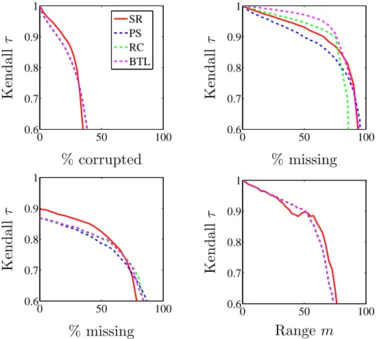
The first synthetic dataset consists of a matrix of pairwise comparisons derived from a given ranking of nitems with uniform, randomly distributed corrupted or missing entries. A second synthetic dataset consists of a full matrix of pairwise comparisons derived from a given ranking of nitems, with added “local” noise on the similarity between nearby items. Specifically, given a positive integer m, we let Ci,j = 1 if i < j−m, Ci,j ∼ Unif[−1,1] if |i−j| ≤m, and Ci,j =−1 ifi > j+m. In Figure 2, we measure the Kendallτ correlation coefficient between the true ranking and the retrieved ranking, when varying either the percentage of corrupted comparisons or the percentage of missing comparisons. Kendall’sτ counts the number of agreeing pairs minus the number of disagreeing pairs between two rankings, scaled by the total number of pairs, so that it takes values between -1 and 1. Experiments were performed with n = 100 and reported Kendall τ values were averaged over 50 experiments, with standard deviation less than 0.02 for points of interest (i.e., with Kendall τ >0.8).
Results suggest that SerialRank (SR, full red line) produces more accurate rankings than point score (PS, (Wauthier et al., 2013) dashed blue line), Rank Centrality (RC (Ne-gahban et al., 2012) dashed green line), and maximum likelihood (BTL (Bradley and Terry, 1952), dashed magenta line) in regimes with limited amount of corrupted and missing com-parisons. In particular SerialRank seems more robust to corrupted comcom-parisons. On the other hand, the performance deteriorates more rapidly in regimes with very high number of corrupted/missing comparisons. For a more exhaustive comparison of SerialRank to state-of-the art ranking algorithms, we refer the interested reader to a recent paper by Cu-curingu (2015), which introduces another ranking algorithm called SyncRank, and provides extensive numerical experiments.
6.2 Real Datasets
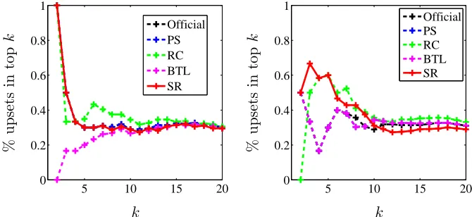
The first real dataset consists of pairwise comparisons derived from outcomes in the Top-Coder algorithm competitions. We collected data from 103 competitions among 2742 coders over a period of about one year. Pairwise comparisons are extracted from the ranking of each competition and then averaged for each pair. TopCoder maintains ratings for each participant, updated in an online scheme after each competition, which were also included in the benchmarks. To measure performance in Figure 3, we compute the percentage of upsets (i.e. comparisons disagreeing with the computed ranking), which is closely related to the Kendallτ (by an affine transformation if comparisons were coming from a consistent ranking). We refine this metric by considering only the participants appearing in the top k, for various values ofk, i.e. computing
lk= 1 |Ck|
X
i,j∈Ck
whereC are the pairs (i, j) that are compared and such thati, jare both ranked in the top k, and r(i) is the rank of i. Up to scaling, this is the loss considered in (Kenyon-Mathieu and Schudy, 2007).
This experiment shows that SerialRank gives competitive results with other ranking algorithms. Notice that rankings could probably be refined by designing a similarity matrix taking into account the specific nature of the data.
Table 1: Ranking of teams in the England premier league season 2013-2014.
Official Row-sum RC BTL SerialRank Semi-Supervised
Man City (86) Man City Liverpool Man City Man City Man City Liverpool (84) Liverpool Arsenal Liverpool Chelsea Chelsea Chelsea (82) Chelsea Man City Chelsea Liverpool Liverpool Arsenal (79) Arsenal Chelsea Arsenal Arsenal Everton Everton (72) Everton Everton Everton Everton Arsenal Tottenham (69) Tottenham Tottenham Tottenham Tottenham Tottenham Man United (64) Man United Man United Man United Southampton Man United Southampton (56) Southampton Southampton Southampton Man United Southampton
Stoke (50) Stoke Stoke Stoke Stoke Newcastle
Newcastle (49) Newcastle Newcastle Newcastle Swansea Stoke Crystal Palace (45) Crystal Palace Swansea Crystal Palace Newcastle West Brom Swansea (42) Swansea Crystal Palace Swansea West Brom Swansea West Ham (40) West Brom West Ham West Brom Hull Crystal Palace Aston Villa (38) West Ham Hull West Ham West Ham Hull
Sunderland (38) Aston Villa Aston Villa Aston Villa Cardiff West Ham Hull (37) Sunderland West Brom Sunderland Crystal Palace Fulham
West Brom (36) Hull Sunderland Hull Fulham Norwich
Norwich (33) Norwich Fulham Norwich Norwich Sunderland Fulham (32) Fulham Norwich Fulham Sunderland Aston Villa Cardiff (30) Cardiff Cardiff Cardiff Aston Villa Cardiff
6.3 Semi-Supervised Ranking
7. Conclusion
We have formulated the problem of ranking from pairwise comparisons as a seriation prob-lem, i.e. the problem of ordering from similarity information. By constructing an adequate similarity matrix, we applied a spectral relaxation for seriation to a variety of synthetic and real ranking datasets, showing competitive and in some cases superior performance com-pared to classical methods, especially in low noise environments. We derived performance bounds for this algorithm in the presence of corrupted and missing (ordinal) comparisons showing that SerialRank produces state-of-the art results for ranking based on ordinal com-parisons, e.g. showing exact reconstruction w.h.p. when only O(√n) comparisons are missing. On the other hand, performance deteriorates when only a small fraction of com-parisons are observed, or in the presence of very high noise. In this scenario, we showed that local ordering errors can be bounded if the number of samples is of orderO(n1.5polylog(n)) which is significantly above the optimal bound of O(nlogn).
A few questions thus remain open, which we pose as future research directions. First of all, from a theoretical perspective, is it possible to obtain an`∞bound on local perturbations of the ranking using only O(npolylog(n)) sampled pairs? Or, on the contrary, can we find a lower bound for spectral algorithms (i.e. perturbation arguments) imposing more than Ω(npolylog(n)) sampled pairs? Note that those questions hold for all current spectral ranking algorithms.
Another line of research concerns the generalization of spectral ordering methods to more flexible settings, e.g., enforcing structural or a priori constraints on the ranking. Hierarchical ranking, i.e. running the spectral algorithm on increasingly refined subsets of the original data should be explored too. Early experiments suggests this works quite well, but no bounds are available at this point.
Finally, it would be interesting to investigate how similarity measures could be tuned for specific applications in order to improve SerialRank predictive power, for instance to take into account more information than win/loss in sports tournaments. Additional experiments in this vein can be found in Cucuringu (2015).
Appendix A.
We now detail several complementary technical results.
A.1 Exact recovery results with missing entries
Here, as in Section 4, we study the impact of one missing comparison on SerialRank, then extend the result to multiple missing comparisons.
Proposition 25 Given pairwise comparisons Cs,t ∈ {−1,0,1} between items ranked ac-cording to their indices, suppose only one comparison Ci,j is missing, with j−i >1 (i.e., Ci,j = 0), then Smatch defined in (3) remains strict-R and the point score vector remains strictly monotonic.
matrixSmatch (respectively ˆS when the similarity is computed from observations). We first study the impact of the missing comparison Ci,j fori < j on the point score vector ˆw. We have
ˆ wi=
n X
k=1 ˆ Ck,i=
n X
k=1
Ck,i+ ˆCj,i−Cj,i=wi+ 1,
similarly ˆwj =wj−1, whereas fork=6 i, j, ˆwk=wk. Hence,wis still strictly increasing ifj > i+ 1. Ifj=i+ 1 there is a tie betweenwi andwi+1. Now we show that the similarity matrix defined in (3) is an R-matrix. Writing ˆS in terms ofS, we get
[ ˆCCˆT]i,t = X
k6=j
ˆ Ci,kCt,kˆ
+ ˆCi,jCt,jˆ =X k6=j
(Ci,kCt,k) =
[CCT]i,t−1 ift < j
CCT
i,t+ 1 ift > j. We thus get
ˆ Si,t =
Si,t−12 ift < j Si,t+12 ift > j,
(remember there is a factor 1/2 in the definition ofS). Similarly we get for anyt6=i
ˆ Sj,t=
Sj,t+12 ift < i Sj,t−1
2 ift > i. Finally, for the single corrupted index pair (i, j), we get
ˆ Si,j = 1
2
n+ X
k6=i,j
ˆ Ci,kCj,kˆ
+ ˆCi,iCj,iˆ + ˆCi,jCj,jˆ
=Si,j−0 + 0 =Si,j.
For all other coefficients (s, t) such that s, t 6= i, j, we have ˆSs,t = Ss,t. Meaning all rows or columns outside of i, j are left unchanged. We first observe that these last equations, together with our assumption thatj−i >2, mean that
ˆ
Ss,t ≥Ss+1,tˆ and Ss,t+1ˆ ≥Ss,t,ˆ for any s < t
so ˆS remains an R-matrix. To show uniqueness of the retrieved order, we need j−i >1. Indeed, whenj−i >1 all theseR constraints are strict, which means that ˆS is still a strict R-matrix, hence the desired result.
We can extend this result to the case where multiple comparisons are missing.
Proposition 26 Given pairwise comparisons Cs,t ∈ {−1,0,1} between items ranked ac-cording to their indices, suppose m comparisons indexed (i1, j1), . . . ,(im, jm) are missing, i.e.,Cil,jj = 0 for i=l, . . . , m. If the following condition (26) holds true,
ProofProceed similarly as in the proof of Proposition 13, except that shifts are divided by two.
We also get the following corollary.
Corollary 27 Given pairwise comparisonsCs,t∈ {−1,0,1}between items ranked according to their indices, suppose m comparisons indexed (i1, j1), . . . ,(im, jm) are either corrupted or missing. If condition (7) holds true then Smatch defined in (3) remains strict-R.
Proof Proceed similarly as the proof of Proposition 13, except that shifts are divided by two for missing comparisons.
A.2 Standard theorems and technical lemmas used in spectral perturbation analysis (section 5)
We first recall Weyl’s inequality and a simplified version of Davis-Kahan theorem which can be found in (Stewart and Sun, 1990; Stewart, 2001; Yu et al., 2015).
Theorem 28 (Weyl’s inequality) Consider a symmetric matrix A with eigenvalues λ1, . . . , λn and A˜ a symmetric perturbation of A with eigenvalues λ˜1, . . . ,λ˜n,
max i |
˜
λi−λi| ≤ kA˜−Ak2.
Theorem 29 (Variant of Davis-Kahan theorem (Corollary 3 Yu et al., 2015))Let A,A˜ ∈ Rn be symmetric, with eigenvalues λ
1 ≤. . . ≤λn and λ˜1 ≤ . . . ≤ ˜λn respectively. Fix j ∈ {1, . . . , n}, and assume that min(λj−λj−1, λj+1−λj)>0, where λn+1 := ∞ and λ0:=−∞. If v,˜v∈Rn satisfy Av =λjv and A˜v˜= ˜λjv˜, then
sin Θ(˜v, v)≤ 2kA˜−Ak2
min(λj−λj−1, λj+1−λj) .
Moreover, if ˜vTv≥0, then
k˜v−vk2 ≤
2√2kA˜−Ak2 min(λj−λj−1, λj+1−λj)
.
When analyzing the perturbation of the Fiedler vector f, we may always reverse the sign of ˜f such that ˜fTf ≥0 and obtain
kf˜−fk2≤
2√2kL˜−Lk2 min(λ2−λ1, λ3−λ2)
.
Lemma 30 Let r >0, for every µ∈(0,1)and n large enough, if q > µ2(2plog−4n1)4n, then
k( ˜S−S)fk∞≤
3µn3/2
√ logn