Positive Semidefinite Metric Learning Using Boosting-like Algorithms
Chunhua Shen [email protected]
The University of Adelaide Adelaide, SA 5005, Australia
Junae Kim [email protected]
NICTA, Canberra Research Laboratory Locked Bag 8001
Canberra, ACT 2601, Australia
Lei Wang [email protected]
University of Wollongong
Wollongong, NSW 2522, Australia
Anton van den Hengel [email protected]
The University of Adelaide Adelaide, SA 5005, Australia
Editors: S¨oren Sonnenburg, Francis Bach, Cheng Soon Ong
Abstract
The success of many machine learning and pattern recognition methods relies heavily upon the identification of an appropriate distance metric on the input data. It is often beneficial to learn such a metric from the input training data, instead of using a default one such as the Euclidean distance. In this work, we propose a boosting-based technique, termed BOOSTMETRIC, for learning a quadratic Mahalanobis distance metric. Learning a valid Mahalanobis distance metric requires enforcing the constraint that the matrix parameter to the metric remains positive semidefinite. Semidefinite programming is often used to enforce this constraint, but does not scale well and is not easy to implement. BOOSTMETRICis instead based on the observation that any positive semidefinite ma-trix can be decomposed into a linear combination of trace-one rank-one matrices. BOOSTMETRIC thus uses rank-one positive semidefinite matrices as weak learners within an efficient and scalable boosting-based learning process. The resulting methods are easy to implement, efficient, and can accommodate various types of constraints. We extend traditional boosting algorithms in that its weak learner is a positive semidefinite matrix with trace and rank being one rather than a classifier or regressor. Experiments on various data sets demonstrate that the proposed algorithms compare favorably to those state-of-the-art methods in terms of classification accuracy and running time.
Keywords: Mahalanobis distance, semidefinite programming, column generation, boosting,
La-grange duality, large margin nearest neighbor
1. Introduction
Vemuri, 2007; Xing et al., 2002; Bar-Hillel et al., 2005; Boiman et al., 2008; Frome et al., 2007) amongst a host of others.
The Euclidean distance has been shown to be effective in a wide variety of circumstances. Boiman et al. (2008), for instance, showed that in generic object recognition with local features,
kNN with a Euclidean metric can achieve comparable or better accuracy than more sophisticated
classifiers such as support vector machines (SVMs). The Mahalanobis distance represents a gen-eralization of the Euclidean distance, and offers the opportunity to learn a distance metric directly from the data. This learned Mahalanobis distance approach has been shown to offer improved per-formance over Euclidean distance-based approaches, and was particularly shown by Wang et al. (2010b) to represent an improvement upon the method of Boiman et al. (2008). It is the prospect of a significant performance improvement from fundamental machine learning algorithms which inspires the approach presented here.
If we let ai,i=1,2· · ·, represent a set of points in RD, then the Mahalanobis distance, or
Gaussian quadratic distance, between two points is
kai−ajkX= q
(ai−aj)⊤X(ai−aj),
where X<0 is a positive semidefinite (p.s.d.) matrix. The Mahalanobis distance is thus param-eterized by a p.s.d. matrix, and methods for learning Mahalanobis distances are therefore often framed as constrained semidefinite programs. The approach we propose here, however, is based on boosting, which is more typically used for learning classifiers. The primary motivation for the boosting-based approach is that it scales well, but its efficiency in dealing with large data sets is also advantageous. The learning of Mahalanobis distance metrics represents a specific application of a more general method for matrix learning which we present below.
We are interested here in the case where the training data consist of a set of constraints upon the relative distances between data points,
I={(ai,aj,ak)|disti j<distik}, (1)
where disti j measures the distance between ai and aj. Each such constraint implies that “ai is
closer to aj than ai is to ak”. Constraints such as these often arise when it is known that aiand aj
belong to the same class of data points while ai,ak belong to different classes. These comparison
constraints are thus often much easier to obtain than either the class labels or distances between data elements (Schultz and Joachims, 2003). For example, in video content retrieval, faces extracted from successive frames at close locations can be safely assumed to belong to the same person, without requiring the individual to be identified. In web search, the results returned by a search engine are ranked according to the relevance, an ordering which allows a natural conversion into a set of constraints.
The problem of learning a p.s.d. matrix such as X can be formulated in terms of estimating a
projection matrix L where X=LL⊤. This approach has the advantage that the p.s.d. constraint
is enforced through the parameterization, but the disadvantage is that the relationship between the distance measure and the parameter matrix is less direct. In practice this approach has lead to local, rather than globally optimal solutions, however (see Goldberger et al., 2004 for example).
semidefiniteness of X during the course of learning. Standard approaches such as interior-point (IP) Newton methods need to calculate the Hessian. This typically requires O(D4)storage and has worst-case computational complexity of approximately O(D6.5)where D is the size of the p.s.d. matrix. This is prohibitive for many real-world problems. An alternating projected (sub-)gradient approach is adopted in Weinberger et al. (2005), Xing et al. (2002) and Globerson and Roweis (2005). The disadvantages of this algorithm, however, are: 1) it is not easy to implement; 2) many parameters are involved; 3) usually it converges slowly.
We propose here a method for learning a p.s.d. matrix labeled BOOSTMETRIC. The method
is based on the observation that any positive semidefinite matrix can be decomposed into a
lin-ear positive combination of trace-one rank-one matrices. The weak llin-earner in BOOSTMETRIC is
thus a trace-one rank-one p.s.d. matrix. The proposed BOOSTMETRICalgorithm has the following
desirable properties:
1. BOOSTMETRICis efficient and scalable. Unlike most existing methods, no semidefinite pro-gramming is required. At each iteration, only the largest eigenvalue and its corresponding eigenvector are needed.
2. BOOSTMETRICcan accommodate various types of constraints. We demonstrate the use of the method to learn a Mahalanobis distance on the basis of a set of proximity comparison constraints.
3. Like AdaBoost, BOOSTMETRICdoes not have any parameter to tune. The user only needs to
know when to stop. Also like AdaBoost it is easy to implement. No sophisticated optimiza-tion techniques are involved. The efficacy and efficiency of the proposed BOOSTMETRICis demonstrated on various data sets.
4. We also propose a totally-corrective version of BOOSTMETRIC. As in TotalBoost (Warmuth
et al., 2006) the weights of all the selected weak learners (rank-one matrices) are updated at each iteration.
Both the stage-wise BOOSTMETRICand totally-corrective BOOSTMETRICmethods are very
easy to implement.
The primary contributions of this work are therefore as follows: 1) We extend traditional boost-ing algorithms such that each weak learner is a matrix with the trace and rank of one—which must be positive semidefinite—rather than a classifier or regressor; 2) The proposed algorithm can be used to solve many semidefinite optimization problems in machine learning and computer vision. We demonstrate the scalability and effectiveness of our algorithms on metric learning. Part of this work appeared in Shen et al. (2008, 2009). More theoretical analysis and experiments are included in this version. Next, we review some relevant work before we present our algorithms.
1.1 Related Work
the neighborhood structure of the data set (He et al., 2005). Essentially, LPP linearly approximates the eigenfunctions of the Laplace Beltrami operator on the underlying manifold. The connection between LPP and LDA is also revealed in He et al. (2005). Wang et al. (2010a) extended LPP to supervised multi-label classification. Relevant component analysis (RCA) (Bar-Hillel et al., 2005) learns a metric from equivalence constraints. RCA can be viewed as extending LDA by incorpo-rating must-link constraints and cannot-link constraints into the learning procedure. Each of these methods may be seen as devising a linear projection from the input space to a lower-dimensional output space. If this projection is characterized by the matrix L, then note that these methods may be related to the problem of interest here by observing X=LL⊤. This typically implies that X is rank-deficient.
Recently, there has been significant research interest in supervised distance metric learning using side information that is typically presented in a set of pairwise constraints. Most of these methods, although appearing in different formats, share a similar essential idea: to learn an optimal dis-tance metric by keeping training examples in equivalence constraints close, and at the same time, examples in in-equivalence constraints well separated. Previous work of Xing et al. (2002), Wein-berger et al. (2005), Jian and Vemuri (2007), GoldWein-berger et al. (2004), Bar-Hillel et al. (2005) and Schultz and Joachims (2003) fall into this category. The requirement that X must be p.s.d. has led to the development of a number of methods for learning a Mahalanobis distance which rely upon constrained semidefinite programing. This approach has a number of limitations, however, which we now discuss with reference to the problem of learning a p.s.d. matrix from a set of constraints upon pairwise-distance comparisons. Relevant work on this topic includes Bar-Hillel et al. (2005), Xing et al. (2002), Jian and Vemuri (2007), Goldberger et al. (2004), Weinberger et al. (2005) and Globerson and Roweis (2005) amongst others.
Xing et al. (2002) first proposed the idea of learning a Mahalanobis metric for clustering using convex optimization. The inputs are two sets: a similarity set and a dis-similarity set. The algorithm maximizes the distance between points in the dis-similarity set under the constraint that the distance between points in the similarity set is upper-bounded. Neighborhood component analysis (NCA) (Goldberger et al., 2004) and large margin nearest neighbor (LMNN) (Weinberger et al., 2005) learn a metric by maintaining consistency in data’s neighborhood and keep a large margin at the boundaries of different classes. It has been shown in Weinberger and Saul (2009); Weinberger et al. (2005) that LMNN delivers the state-of-the-art performance among most distance metric learning algorithms. Information theoretic metric learning (ITML) learns a suitable metric based on infor-mation theoretics (Davis et al., 2007). To partially alleviate the heavy computation of standard IP Newton methods, Bregman’s cyclic projection is used in Davis et al. (2007). This idea is extended in Wang and Jin (2009), which has a closed-form solution and is computationally efficient.
semidefinite kernel learning, they designed a matrix exponentiated gradient method to optimize von Neumann divergence based objective functions. At each iteration of matrix exponentiated gradient, a full eigen-decomposition is needed. In contrast, we only need to find the leading eigenvector.
The approach proposed here is directly inspired by the LMNN proposed in Weinberger and Saul (2009); Weinberger et al. (2005). Instead of using the hinge loss, however, we use the exponential loss and logistic loss functions in order to derive an AdaBoost-like (or LogitBoost-like) optimization procedure. In theory, any differentiable convex loss function can be applied here. Hence, despite similar purposes, our algorithm differs essentially in the optimization. While the formulation of
LMNN looks more similar to SVMs, our algorithm, termed BOOSTMETRIC, largely draws upon
AdaBoost (Schapire, 1999).
Column generation was first proposed by Dantzig and Wolfe (1960) for solving a particular form of structured linear program with an extremely large number of variables. The general idea of column generation is that, instead of solving the original large-scale problem (master problem), one works on a restricted master problem with a reasonably small subset of the variables at each step. The dual of the restricted master problem is solved by the simplex method, and the optimal dual solution is used to find the new column to be included into the restricted master problem. LP-Boost (Demiriz et al., 2002) is a direct application of column generation in boosting. Significantly, LPBoost showed that in an LP framework, unknown weak hypotheses can be learned from the dual although the space of all weak hypotheses is infinitely large. Shen and Li (2010) applied column generation to boosting with general loss functions. It is these results that underpin BOOSTMETRIC. The remaining content is organized as follows. In Section 2 we present some preliminary math-ematics. In Section 3, we show the main results. Experimental results are provided in Section 4.
2. Preliminaries
We introduce some fundamental concepts that are necessary for setting up our problem. First, the notation used in this paper is as follows.
2.1 Notation
Throughout this paper, a matrix is denoted by a bold upper-case letter (X); a column vector is denoted by a bold lower-case letter (xxx). The ith row of X is denoted by Xi:and the ith column X:i.
111 and 000 are column vectors of 1’s and 0’s, respectively. Their size should be clear from the context. We denote the space of D×D symmetric matrices bySD, and positive semidefinite matrices bySD
+.
Tr(·) is the trace of a symmetric matrix andhX,Zi=Tr(XZ⊤) =∑i jXi jZi j calculates the inner
product of two matrices. An element-wise inequality between two vectors like uuu≤vvv means ui≤vi
for all i. We use X<0 to indicate that matrix X is positive semidefinite. For a matrix X∈SD, the
following statements are equivalent: 1) X<0 (X∈SD
+); 2) All eigenvalues of X are nonnegative
(λi(X)≥0, i=1,· · ·,D); and 3)∀uuu∈RD, uuu⊤Xuuu≥0.
2.2 A Theorem on Trace-one Semidefinite Matrices
Definition 1 For any positive integer m, given a set of points{xxx1, ...,xxxm}in a real vector or matrix space Sp, the convex hull of Sp spanned by m elements in Sp is defined as:
Convm(Sp) =
n
∑m
i=1wixxxi
wi≥0,∑mi=1wi=1,xxxi∈Sp
o
.
Define the linear convex span of Sp as:1
Conv(Sp) =[
m
Convm(Sp) =
n
∑m
i=1wixxxi
wi≥0,∑mi=1wi=1,xxxi∈Sp,m∈Z+
o
.
HereZ+denotes the set of all positive integers.
Definition 2 Let us defineΓ1to be the space of all positive semidefinite matrices X∈SD+with trace equaling one:
Γ1={X|X<0,Tr(X) =1};
andΨ1to be the space of all positive semidefinite matrices with both trace and rank equaling one:
Ψ1={Z|Z<0,Tr(Z) =1,Rank(Z) =1}.
We also defineΓ2as the convex hull ofΨ1, that is,
Γ2=Conv(Ψ1).
Lemma 3 LetΨ2be a convex polytope defined asΨ2={λλλ∈RD|λk≥0,∀k=0,· · ·,D,∑Dk=1λk=
1}, then the points with only one element equaling one and all the others being zeros are the extreme
points (vertexes) ofΨ2. All the other points can not be extreme points.
Proof Without loss of generality, let us consider such a pointλλλ′={1,0,· · ·,0}. Ifλλλ′ is not an extreme point of Ψ2, then it must be possible to express it as a convex combination of a set of
other points in Ψ2: λλλ′ =∑mi=1wiλλλ
i
, wi >0, ∑mi=1wi=1 andλλλ i
6
=λλλ′. Then we have equations:
∑m
i=1wiλik=0,∀k=2,· · ·,D. It follows thatλki =0, ∀i and k=2,· · ·,D. That means,λi1=1∀i.
This is inconsistent withλλλi6=λλλ′. Therefore such a convex combination does not exist andλλλ′must be an extreme point. It is trivial to see that anyλλλthat has more than one active element is an convex combination of the above-defined extreme points. So they can not be extreme points.
Theorem 4 Γ1equals toΓ2; that is, Γ1 is also the convex hull ofΨ1. In other words, all Z∈Ψ1,
form the set of extreme points ofΓ1.
Proof It is easy to check that any convex combination∑iwiZi, such that Zi∈Ψ1, resides inΓ1,
with the following two facts: 1) a convex combination of p.s.d. matrices is still a p.s.d. matrix; 2)
Tr ∑iwiZi
=∑iwiTr(Zi) =1.
By denoting λ1≥ · · · ≥λD≥0 the eigenvalues of a Z∈Γ1, we know that λ1≤1 because
∑D
i=1λi=Tr(Z) =1. Therefore, all eigenvalues of Z must satisfy: λi∈[0,1],∀i=1,· · ·,D and
∑D
i λi=1. By looking at the eigenvalues of Z and using Lemma 3, it is immediate to see that a
matrix Z such that Z<0, Tr(Z) =1 and Rank(Z)>1 can not be an extreme point ofΓ1. The only
candidates for extreme points are those rank-one matrices (λ1=1 andλ2,···,D=0). Moreover, it is
not possible that some rank-one matrices are extreme points and others are not because the other two constraints Z<0 and Tr(Z) =1 do not distinguish between different rank-one matrices.
Hence, all Z∈Ψ1form the set of extreme points ofΓ1. Furthermore,Γ1is a convex and compact
set, which must have extreme points. The Krein-Milman Theorem (Krein and Milman, 1940) tells us that a convex and compact set is equal to the convex hull of its extreme points.
This theorem is a special case of the results from Overton and Womersley (1992) in the context of eigenvalue optimization. A different proof for the above theorem’s general version can also be found in Fillmore and Williams (1971).
In the context of semidefinite optimization, what is of interest about Theorem 4 is as follows: it tells us that a bounded p.s.d. matrix constraint X∈Γ1can be equivalently replaced with a set of
constrains which belong toΓ2. At the first glance, this is a highly counterintuitive proposition
be-causeΓ2involves many more complicated constraints. Both wiand Zi(∀i=1,· · ·,m) are unknown
variables. Even worse, m could be extremely (or even infinitely) large. Nevertheless, this is the type of problems that boosting algorithms are designed to solve. Let us give a brief overview of boosting algorithms.
2.3 Boosting
Boosting is an example of ensemble learning, where multiple learners are trained to solve the same problem. Typically a boosting algorithm (Schapire, 1999) creates a single strong learner by incre-mentally adding base (weak) learners to the final strong learner. The base learner has an important impact on the strong learner. In general, a boosting algorithm builds on a user-specified base learn-ing procedure and runs it repeatedly on modified data that are outputs from the previous iterations.
The general form of the boosting algorithm is sketched in Algorithm 1. The inputs to a boosting algorithm are a set of training example xxx, and their corresponding class labels y. The final output is a strong classifier which takes the form
Fwww(xxx) =∑Jj=1wjhj(xxx). (2)
Here hj(·)is a base learner. From Theorem 4, we know that a matrix X∈Γ1can be decomposed as X=∑J
j=1wjZj,Zj∈Γ2. (3)
By observing the similarity between Equations (2) and (3), we may view Zj as a weak classifier
and the matrix X as the strong classifier that we want to learn. This is exactly the problem that boosting methods have been designed to solve. This observation inspires us to solve a special type of semidefinite optimization problem using boosting techniques.
The sparse greedy approximation algorithm proposed by Zhang (2003) is an efficient method for solving a class of convex problems, and achieves fast convergence rates. It has also been shown that boosting algorithms can be interpreted within the general framework of Zhang (2003). The main idea of sequential greedy approximation, therefore, is as follows. Given an initialization uuu0, which
Algorithm 1 The general framework of boosting.
Input: Training data.
Initialize a weight set uuu on the training examples; 1
for j=1,2,· · ·,do 2
···Receive a weak hypothesis hj(·); 3
···Calculate wj>0; 4
···Update uuu. 5
Output: A convex combination of the weak hypotheses: Fwww(xxx) =∑Jj=1wjhj(xxx).
solution uuuiis updated as uuui= (1−λ)uuui−1+λuuuiand the iteration goes on. Clearly, uuuimust remain in the original space. As shown next, our first case, which learns a metric using the hinge loss, greatly resembles this idea.
2.4 Distance Metric Learning Using Proximity Comparison
The process of measuring distance using a Mahalanobis metric is equivalent to linearly transforming the data by a projection matrix L∈RD×d(usually D≥d) before calculating the standard Euclidean
distance:
dist2i j=kL⊤ai−L⊤ajk22= (ai−aj)⊤LL⊤(ai−aj) = (ai−aj)⊤X(ai−aj).
As described above, the problem of learning a Mahalanobis metric can be approached in terms of learning the matrix L, or the p.s.d. matrix X. If X=I, the Mahalanobis distance reduces to the
Euclidean distance. If X is diagonal, the problem corresponds to learning a metric in which different features are given different weights, a.k.a., feature weighting. Our approach is to learn a full p.s.d.
matrix X, however, using BOOSTMETRIC.
In the framework of large-margin learning, we want to maximize the distance between disti j
and distik. That is, we wish to make dist2ik−dist2i j= (ai−ak)⊤X(ai−ak)−(ai−aj)⊤X(ai−aj)as
large as possible under some regularization. To simplify notation, we rewrite the distance between
dist2i j and dist2ikas dist2ik−dist2i j=hAr,Xi,where
Ar= (ai−ak)(ai−ak)⊤−(ai−aj)(ai−aj)⊤, (4)
for r=1,· · ·,|I|and|I|is the size of the set of constraintsI defined in Equation (1).
3. Algorithms
In this section, we define the optimization problems for metric learning. We mainly investigate the cases using the hinge loss, exponential loss and logistic loss functions. In order to derive an efficient optimization strategy, we look at their Lagrange dual problems and design boosting-like approaches for efficiency.
3.1 Learning with the Hinge Loss
Our goal is to derive a general algorithm for p.s.d. matrix learning with the hinge loss function. Assume that we want to find a p.s.d. matrix X<0 such that a set of constraints
are satisfied as well as possible. Here Ar is as defined in (4). These constraints need not all be
strictly satisfied and thus we define the marginρr=hAr,Xi,∀r.
Putting it into the maximum margin learning framework, we want to minimize the following trace norm regularized objective function:∑rF(hAr,Xi)+v Tr(X),with F(·)a convex loss function
and v a regularization constant. Here we have used the trace norm regularization. Of course a
Frobenius norm regularization term can also be used here. Minimizing the Frobenius norm||X||2
F,
which is equivalent to minimize theℓ2norm of the eigenvalues of X, penalizes a solution that is far
away from the identity matrix. With the hinge loss, we can write the optimization problem as:
max
ρ,X,ξξξ ρ−v∑
|I|
r=1ξr,s.t.:hAr,Xi ≥ρ−ξr,∀r; X<0,Tr(X) =1;ξξξ≥000. (5)
Here Tr(X) =1 removes the scale ambiguity because the distance inequalities are scale invariant.
We can decompose X into: X=∑J
j=1wjZj,with wj >0, Rank(Zj) =1 and Tr(Zj) =1,∀j.
So we have
hAr,Xi=Ar,∑Jj=1wjZj
=∑Jj=1wjAr,Zj
=∑Jj=1wjHr j=Hr:www,∀r. (6)
Here Hr j is a shorthand for Hr j=
Ar,Zj
. Clearly, Tr(X) =111⊤www. Using Theorem 4, we replace
the p.s.d. conic constraint in the primal (5) with a linear convex combination of rank-one unitary matrices: X=∑jwjZj,and 111⊤www=1. Substituting X in (5), we have
max
ρ,www,ξξξρ−v∑
|I|
r=1ξr,s.t.: Hr:www≥ρ−ξr,(r=1, . . . ,|I|);www≥000,111
⊤www=1;ξξξ≥000. (7)
The Lagrange dual problem of the above linear programming problem (7) is easily derived:
min
π,uuu πs.t.:∑
|I|
r=1urHr:≤π111
⊤;111⊤uuu=1,000≤uuu≤v111.
We can then use column generation to solve the original problem iteratively by looking at both the primal and dual problems. See Shen et al. (2008) for the algorithmic details. In this work we are more interested in smooth loss functions such as the exponential loss and logistic loss, as presented in the sequel.
3.2 Learning with the Exponential Loss
By employing the exponential loss, we want to optimize
min
X,ρρρ log ∑
|I|
r=1exp(−ρr)
+v Tr(X)
s.t.:ρr=hAr,Xi,r=1,· · ·,|I|,X<0. (8)
We now derive the Lagrange dual of the problem that we are interested in. The original problem (8) now becomes
min
ρρρ,www log ∑
|I|
r=1exp(−ρr)
+v111⊤www
s.t.:ρr=Hr:www,r=1,· · ·,|I|; www≥000. (9)
We have used the Equation (6). In order to derive its dual, we write its Lagrangian
L(www,ρρρ,uuu) =log ∑r|I=|1exp(−ρr)
+v111⊤www+∑|rI=|1ur(ρr−Hr:www)−ppp⊤www,
with ppp≥0. The dual problem is obtained by finding the saddle point of L; that is, supuuuinfwww,ρρρL.
inf
w
ww,ρρρL=infρρρ
L1
z }| {
log ∑|rI=|1exp(−ρr)
+uuu⊤ρρρ+inf
www
L2
z }| {
(v111⊤−∑|rI=|1urHr:−ppp⊤)www (10)
=−∑|rI=|1urlog ur.
The infimum of L1is found by setting its first derivative to zero and we have:
inf
ρρρ L1=
(
−∑rurlog ur if uuu≥000,111⊤uuu=1,
−∞ otherwise.
The infimum is Shannon entropy. L2is linear in www, hence it must be 000. It leads to
∑|I|
r=1urHr:≤v111⊤. (11)
The Lagrange dual problem of (9) is an entropy maximization problem, which writes
max
uuu −∑ |I|
r=1urlog ur,s.t.: uuu≥000,111⊤uuu=1,and (11). (12)
Weak and strong duality hold under mild conditions (Boyd and Vandenberghe, 2004). That means, one can usually solve one problem from the other. The KKT conditions link the optimal between these two problems. In our case, it is
u⋆r= exp(−ρ
⋆
r)
∑|I|
k=1exp(−ρ⋆k)
,∀r. (13)
While it is possible to devise a totally-corrective column generation based optimization proce-dure for solving our problem as the case of LPBoost (Demiriz et al., 2002), we are more interested in considering one-at-a-time coordinate-wise descent algorithms, as the case of AdaBoost (Schapire, 1999). Let us start from some basic knowledge of column generation because our coordinate descent strategy is inspired by column generation.
If we know all the bases Zj(j=1. . .J)and hence the entire matrix H is known. Then either
the bases: the possibility of Z is infinite. In convex optimization, column generation is a technique that is designed for solving this difficulty.
Column generation was originally advocated for solving large scale linear programs (L¨ubbecke and Desrosiers, 2005). Column generation is based on the fact that for a linear program, the number of non-zero variables of the optimal solution is equal to the number of constraints. Therefore, although the number of possible variables may be large, we only need a small subset of these in the optimal solution. For a general convex problem, we can use column generation to obtain an
approximate solution. It works by only considering a small subset of the entire variable set. Once
it is solved, we ask the question:“Are there any other variables that can be included to improve the solution?”. So we must be able to solve the subproblem: given a set of dual values, one either identifies a variable that has a favorable reduced cost, or indicates that such a variable does not exist. Essentially, column generation finds the variables with negative reduced costs without explicitly enumerating all variables.
Instead of directly solving the primal problem (9), we find the most violated constraint in the dual (12) iteratively for the current solution and adds this constraint to the optimization problem. For this purpose, we need to solve
ˆ
Z=argmaxZ
n
∑|I|
r=1ur
Ar,Z
,s.t.: Z∈Ψ1
o
. (14)
We discuss how to efficiently solve (14) later. Now we move on to derive a coordinate descent optimization procedure.
3.3 Coordinate Descent Optimization
We show how an AdaBoost-like optimization procedure can be derived.
3.3.1 OPTIMIZING FORwj
Since we are interested in the one-at-a-time coordinate-wise optimization, we keep w1,w2, . . . ,wj−1
fixed when solving for wj. The cost function of the primal problem is (in the following derivation,
we drop those terms irrelevant to the variable wj)
Cp(wj) =log
∑|I|
r=1exp(−ρrj−1)·exp(−Hr jwj)
+vwj.
Clearly, Cpis convex in wjand hence there is only one minimum that is also globally optimal. The
first derivative of Cpw.r.t. wjvanishes at optimality, which results in
∑|I|
r=1(Hr j−v)urj−1exp(−wjHr j) =0. (15)
If Hr jis discrete, such as{+1,−1}in standard AdaBoost, we can obtain a closed-form solution
similar to AdaBoost. Unfortunately in our case, Hr jcan be any real value. We instead use bisection
to search for the optimal wj. The bisection method is one of the root-finding algorithms. It
repeat-edly divides an interval in half and then selects the subinterval in which a root exists. Bisection is a simple and robust, although it is not the fastest algorithm for root-finding. Algorithm 2 gives the bisection procedure. We have used the fact that the l.h.s. of (15) must be positive at wl. Otherwise
Algorithm 2 Bisection search for wj.
Input: An interval[wl,wu]known to contain the optimal value of wjand convergence
toleranceε>0.
repeat 1
···wj=0.5(wl+wu);
2
···if l.h.s. of (15)>0 then
3
wl=wj;
4
else 5
wu=wj.
6
until wu−wl<ε; 7
Output: wj.
3.3.2 UPDATINGuuu
The rule for updating uuu can be easily obtained from (13). At iteration j, we have
urj∝exp(−ρrj)∝urj−1exp(−Hr jwj),and∑r|I=|1urj=1,
derived from (13). So once wjis calculated, we can update uuu as
urj=u
j−1
r exp(−Hr jwj)
z ,r=1, . . . ,|I|, (16)
where z is a normalization factor so that∑|rI=|1urj=1. This is exactly the same as AdaBoost. 3.4 The Base Learning Algorithm
In this section, we show that the optimization problem (14) can be exactly and efficiently solved using eigenvalue-decomposition (EVD).
From Z<0 and Rank(Z) =1, we know that Z has the format: Z=vvvvvv⊤, vvv∈RD; and Tr(Z) =1
meanskvvvk2=1. We have
∑|I|
r=1urAr,Z
=vvv ∑|rI=|1urAr
vvv⊤.
By denoting
ˆ
A=∑|rI=|1urAr, (17)
the base learning optimization equals:
max
vvv vvv
⊤Avvvˆ ,s.t.:kvvvk
2=1. (18)
It is clear that the largest eigenvalue of ˆA,λmax(Aˆ), and its corresponding eigenvector vvv1 gives the
solution to the above problem. Note that ˆA is symmetric.
λmax(Aˆ)is also used as one of the stopping criteria of the algorithm. Form the condition (11),
λmax(Aˆ)<v means that we are not able to find a new base matrix ˆZ that violates (11)—the algorithm
Algorithm 3 Positive semidefinite matrix learning with stage-wise boosting.
Input:
• Training set triplets(ai,aj,ak)∈ I; Compute Ar,r=1,2,· · ·,using (4).
• J: maximum number of iterations;
• (optional) regularization parameter v; We may simply set v to a very small value, for example, 10−7.
Initialize: u0r= |I1|,r=1· · · |I|;
1
for j=1,2,· · ·,J do 2
···Find a new base Zj by finding the largest eigenvalue (λmax(Aˆ)) and its eigenvector of 3
ˆ
A in (17);
···if λmax(Aˆ)<v then
4
break (converged);
5
···Compute wjusing Algorithm 2; 6
···Update uuu to obtain ur,rj =1,· · · |I|using (16);
7
Output: The final p.s.d. matrix X∈RD×D, X=∑J
j=1wjZj.
Eigenvalue decompositions is one of the main computational costs in our algorithm. There
are approximate eigenvalue solvers, which guarantee that for a symmetric matrix U and any ε>
0, a vector vvv is found such that vvv⊤Uvvv≥λmax−ε. To approximately find the largest eigenvalue
and eigenvector can be very efficient using Lanczos or power method. We can use the MATLAB
functioneigsto calculate the largest eigenvector, which calls mex files of ARPACK. ARPACK is
a collection of Fortran subroutines designed to solve large scale eigenvalue problems. When the input matrix is symmetric, this software uses a variant of the Lanczos process called the implicitly restarted Lanczos method.
Another way to reduce the time for computing the leading eigenvector is to compute an approx-imate EVD by a fast Monte Carlo algorithm such as the linear time SVD algorithm developed in Drineas et al. (2004).
We summarize our main algorithmic results in Algorithm 3.
3.5 Learning with the Logistic Loss
We have considered the exponential loss in the last content. The proposed framework is so general that it can also accommodate other convex loss functions. Here we consider the logistic loss, which penalizes mis-classifications with more moderate penalties than the exponential loss. It is believed on noisy data, the logistic loss may achieve better classification performance.
With the same settings as in the case of the exponential loss, we can write our optimization problem as
min
ρρρ,www ∑
|I|
r=1logit(ρr) +v1⊤www
Here logit(·) is the logistic loss defined as logit(z) =log(1+exp(−z)). Similarly, we derive its Lagrange dual as
min
u uu ∑
|I|
r=1logit∗(−ur)
s.t.:∑r|I=|1urHr:≤v1⊤,
where logit∗(·)is the Fenchel conjugate function of logit(·), defined as
logit∗(−u) =u log(u) + (1−u)log(1−u),
when 0≤u≤1, and∞otherwise. So the Fenchel conjugate of logit(·)is the binary entropy function. We have reversed the sign of uuu when deriving the dual.
Again, according to the KKT conditions, we have
u⋆r= exp(−ρ
⋆
r)
1+exp(−ρ⋆
r)
, ∀r, (20)
at optimality. From (20) we can also see that u must be in(0,1).
Similarly, we want to optimize the primal cost function in a coordinate descent way. First, let us find the relationship between urjand urj−1. Here j is the iteration index. From (20), it is trivial to
obtain
urj= 1
(1/urj−1−1)exp(Hr jwj) +1
, ∀r. (21)
The optimization of wjcan be solved by looking for the root of
∑|I|
r=1Hr ju j
r−v=0, (22)
where urj is a function of wjas defined in (21).
Therefore, in the case of the logistic loss, to find wj, we modify the bisection search of
Algo-rithm 2:
• Line 3: if l.h.s. o f (22)>0 then . . .
and Line 7 of Algorithm 3:
• Line 7: Update uuu using (21).
3.6 Totally Corrective Optimization
In this section, we derive a totally-corrective version of BOOSTMETRIC, similar to the case of Total-Boost (Warmuth et al., 2006; Shen and Li, 2010) for classification, in the sense that the coefficients of all weak learners are updated at each iteration.
Unlike the stage-wise optimization, here we do not need to keep previous weights of weak learners w1,w2, . . . ,wj−1. Instead, the weights of all the selected weak learners w1,w2, . . . ,wj are
Algorithm 4 Positive semidefinite matrix learning with totally corrective boosting.
Input:
• Training set triplets(ai,aj,ak)∈ I; Compute Ar,r=1,2,· · ·,using (4).
• J: maximum number of iterations;
• Regularization parameter v.
Initialize: u0r= 1
|I|,r=1· · · |I|; 1
for j=1,2,· · ·,J do 2
···Find a new base Zj by finding the largest eigenvalue (λmax(Aˆ)) and its eigenvector of 3
ˆ
A in (17);
···if λmax(Aˆ)<v then
4
break (converged);
5
···Optimize for w1,w2,· · ·,wj by solving the primal problem (9) when the exponential
6
loss is used or (19) when the logistic loss is used;
···Update uuu to obtain urj,r=1,· · · |I|using (13) (exponential loss) or (20) (logistic loss); 7
Output: The final p.s.d. matrix X∈RD×D, X=∑J
j=1wjZj.
to be differentiable with respect to the variables w1,w2, . . . ,wj. Here, we use the exponential loss
function and the logistic loss function. It is possible to use sub-gradient descent methods when a non-smooth loss function like the hinge loss is used.
It is clear that solving for www is a typical convex optimization problem since it has a differentiable
and convex function (9) when the exponential loss is used, or (19) when the logistic loss is used. Hence it can be solved using off-the-shelf gradient-descent solvers like L-BFGS-B (Zhu et al., 1997).
Since all the weights w1,w2, . . . ,wj are updated, urj on r=1. . .|I|need not to be updated but
re-calculated at each iteration j. To calculate urj, we use (13) (exponential loss) or (20) (logistic loss)
instead of (16) or (21) respectively. Totally-corrective BOOSTMETRICmethods are very simple to implement. Algorithm 4 gives the summary of this algorithm. Next, we show the convergence property of Algorithm 4. Formally, we want to show the following theorem.
Theorem 5 Algorithm 4 makes progress at each iteration. In other words, the objective value is decreased at each iteration. Therefore, in the limit, Algorithm 4 solves the optimization problem (9) (or (19)) globally to a desired accuracy.
Proof Let us consider the exponential loss case of problem (9). The proof follows the same
discus-sion for the logistic loss, or any other smooth convex loss function. Assume that the current solution is a finite subset of base learners (rank-one trace-one matrices) and their corresponding linear coef-ficients www. If we add a base matrix ˆZ that is not in the current subset, and the corresponding ˆw=0, then the objective value and the solution must remain unchanged. We can conclude that the current learned base learners and www are the optimal solution already.
holds. Now assume that ˆZ is the base learner found by solving (18), and the convergence condition
λmax(Aˆ)≤v is not satisfied. So, we haveλmax(Aˆ) =
D
∑|I|
r=1urAr,Zˆ
E
>v.
If, after this weak learner ˆZ is added into the primal problem, the primal solution remains
unchanged, that is, the corresponding ˆw=0, then from the optimality condition that L2in (10) must
be zero, we know that ˆp=v−D∑r|I=|1urAr,Zˆ
E
<0. This contradicts the fact the Lagrange multiplier ˆ
p≥0.
We can conclude that after the base learner ˆZ is added into the primal problem, its corresponding
ˆ
w must admit a positive value. It means that one more free variable is added into the problem and
re-solving the primal problem would reduce the objective value. Hence a strict decrease in the objective is guaranteed. So Algorithm 4 makes progress at each iteration.
Furthermore, as the optimization problems involved are all convex, there are no local optimal solutions. Therefore Algorithm 4 is guaranteed to converge to the global solution.
Note that the above proof establishes the convergence of Algorithm 4 but it remains unclear about the convergence rate.
3.7 Multi-pass BOOSTMETRIC
In this section, we show that BOOSTMETRIC can use multi-pass learning to enhance the
perfor-mance.
Our BOOSTMETRICuses training set triplets(ai,aj,ak)∈ I as input for training. The
Maha-lanobis distance metric X can be viewed as a linear transformation in the Euclidean space by project-ing the data usproject-ing matrix L(X=LL⊤). That is, nearest neighbors of samples using Mahalanobis distance metric X are the same as nearest neighbors using Euclidean distance in the transformed space. BOOSTMETRICassumes that the triplets of input training set approximately represent the actual nearest neighbors of samples in the transformed space defined by the Mahalanobis metric.
However, even though the triplets of BOOSTMETRICconsist of nearest neighbors of the original
training samples, generated triplets are not exactly the same as the actual nearest neighbors of train-ing samples in the transformed space by L.
We can refine the results of BOOSTMETRICiteratively, as in the multiple-pass LMNN
(Wein-berger and Saul, 2009): BOOSTMETRIC can estimate the triplets in the transformed space under
a multiple-pass procedure as close to actual triplets as possible. The rule for multi-pass BOOST -METRICis simple. At each pass p (p=1,2,· · ·), we decompose the learned Mahalanobis distance metric Xp−1 of previous pass into transformation matrix Lp. The initial matrix L1 is an identity
matrix. Then we generate the training set triplets from the set of points{L⊤a1, . . . ,L⊤am}where L=L1·L2· · · ·Lp. The final Mahalanobis distance metric X becomes LL⊤in Multi-pass BOOST
-METRIC.
4. Experiments
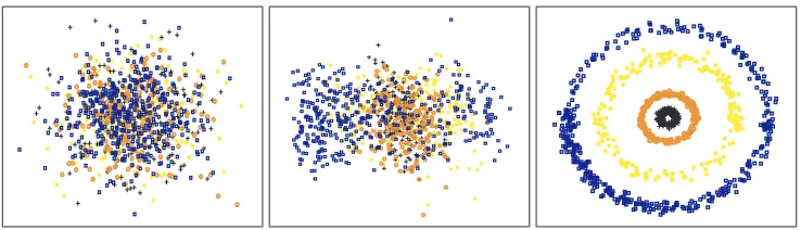
Figure 1: The data are projected into 2D with PCA (left), LDA (middle) and BOOSTMETRIC (right). Both PCA and LDA fail to recover the data structure. The local structure of the data is preserved after projection by BOOSTMETRIC.
4.1 An Illustrative Example
We demonstrate a data visualization problem on an artificial toy data set (concentric circles) in Fig-ure 1. The data set has four classes. The first two dimensions follow concentric circles while the left eight dimensions are all random Gaussian noise. In this experiment, 9000 triplets are generated for training. When the scale of the noise is large, PCA fails find the first two informative dimensions. LDA fails too because clearly each class does not follow a Gaussian distraction and their centers
overlap at the same point. The proposed BOOSTMETRICalgorithm find the informative features.
The eigenvalues of X learned by BOOSTMETRIC are {0.542,0.414,0.007,0,· · ·,0}, which
indi-cates that BOOSTMETRICsuccessfully reveals the data’s underlying 2D structure. We have used
the exponential loss in this experiment.
4.2 Classification on Benchmark Data Sets
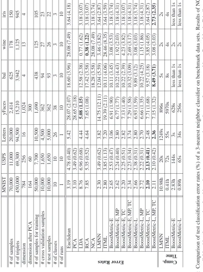
We evaluate BOOSTMETRIC on 7 data sets of different sizes. Some of the data sets have very
high dimensional inputs. We use PCA to decrease the dimensionality before training on these data sets (MNIST, USPS and yFaces). PCA pre-processing helps to eliminate noises and speed up computation. Table 1 summarizes the data sets in detail. We have used USPS and MNIST handwritten digits, Yale face recognition data sets, and a few UCI machine learning data sets.2
Experimental results are obtained by averaging over 10 runs (except for large data sets MNIST and Letter). We randomly split the data sets for each run. We have used the same mechanism to generate training triplets as described in Weinberger et al. (2005). Briefly, for each training point ai, k nearest neighbors that have same labels as yi (targets), as well as k nearest neighbors
that have different labels from yi (imposers) are found. We then construct triplets from ai and its
corresponding targets and imposers. For all the data sets, we have set k=3 (3-nearest-neighbor). We have compared our method against a few methods: RCA (Bar-Hillel et al., 2005), NCA (Goldberger et al., 2004), ITML (Davis et al., 2007) and LMNN (Weinberger et al., 2005). Also in Table 1, “Euclidean” is the baseline algorithm that uses the standard Euclidean distance. The codes for these compared algorithms are downloaded from the corresponding author’s website. Experiment setting for LMNN follows Weinberger et al. (2005). The slack variable parameter for ITML is tuned using
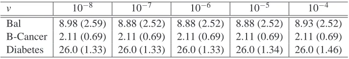
v 10−8 10−7 10−6 10−5 10−4
Bal 8.98 (2.59) 8.88 (2.52) 8.88 (2.52) 8.88 (2.52) 8.93 (2.52)
B-Cancer 2.11 (0.69) 2.11 (0.69) 2.11 (0.69) 2.11 (0.69) 2.11 (0.69)
Diabetes 26.0 (1.33) 26.0 (1.33) 26.0 (1.33) 26.0 (1.34) 26.0 (1.46)
Table 2: Test error (%) of a 3-nearest neighbor classifier with different values of the parameter v. Each experiment is run 10 times. We report the mean and variance. As expected, as long as v is sufficiently small, in a wide range it almost does not affect the final classification performance.
cross validation over the values 0.01,0.1,1,10 as in Davis et al. (2007). For BOOSTMETRIC, we have set v=10−7, the maximum number of iterations J=500.
BOOSTMETRIChas different variants which use 1) the exponential loss (BOOSTMETRIC-E), 2) the logistic loss (BOOSTMETRIC-L), 3) multiple pass evaluation (MP) for updating triplets with the exponential and logistic loss, and 4) two optimization strategies, namely, stage-wise optimization and totally corrective optimization. The experiments are conducted by using Matlab and a C-mex implementation of the L-BFGS-B algorithm.
As reported in Table 1, we can conclude: 1) BOOSTMETRICconsistently improves the
accu-racy of kNN classification using Euclidean distance on most data sets. So learning a Mahalanobis metric based upon the large margin concept indeed leads to improvements in kNN classification. 2) BOOSTMETRIC outperforms other state-of-the-art algorithms in most cases (on 5 out of 7 data sets). LMNN is the second best algorithm on these 7 data sets statistically. LMNN’s results are
consistent with those given in Weinberger et al. (2005). ITML is faster than BOOSTMETRIC on
most large data sets such as MNIST. However it has higher error rates than BOOSTMETRICin our
experiment. 3) NCA can only be run on a few small data sets. In general NCA does not perform well. Initialization is important for NCA because NCA’s objective function is highly non-convex and can only find a local optimum.
In this experiment, LMNN solves for the global optimum (learning X) except for the Wine data
set. When the LMNN solver solves for X on the Wine data set, the error rate is large (20.77%±
14.18%). So instead we have solved for the projection matrix L on Wine. Also note that the number of training data on Iris, Wine and Bal in Weinberger et al. (2005) are different from our experiment. We have used these data sets from UCI. For the experiment on MNIST, if we deskew the handwritten digits data first as in Weinberger and Saul (2009), the final accuracy can be slightly improved. Here we have not deskewed the data.
4.2.1 INFLUENCE OFv
Previously, we claim that the stage-wise version of BOOSTMETRICis parameter-free like AdaBoost.
However, we do have a parameter v. Actually, AdaBoost simply set v=0. The coordinate-wise
gra-dient descent optimization strategy of AdaBoost leads to anℓ1-norm regularized maximum margin
classifier (Rosset et al., 2004). It is shown that AdaBoost minimizes its loss criterion with anℓ1
con-straint on the coefficient vector. Given the similarity of the optimization of BOOSTMETRIC with
AdaBoost, we conjecture that BOOSTMETRIChas the same property. Here we empirically prove
set v from 10−8to 10−4and run BOOSTMETRICon 3 UCI data sets. Table 2 reports the final 3NN classification error with different v. The results are nearly identical.
For the totally corrective version of BOOSTMETRIC, similar results are observed. Actually for LMNN, it was also reported that the regularization parameter does not have a significant impact on the final results in a wide range (Weinberger and Saul, 2009).
4.2.2 COMPUTATIONALTIME
As we discussed, one major issue in learning a Mahalanobis distance is heavy computational cost because of the semidefiniteness constraint.
We have shown the running time of the proposed algorithm in Table 1 for the classification tasks.3 Our algorithm is generally fast. Our algorithm involves matrix operations and an EVD for finding its largest eigenvalue and its corresponding eigenvector. The time complexity of this EVD
is O(D2)with D the input dimensions. We compare our algorithm’s running time with LMNN in
Figure 2 on the artificial data set (concentric circles). Our algorithm is stage-wise BOOSTMETRIC with the exponential loss. We vary the input dimensions from 50 to 1000 and keep the number of triplets fixed to 250. LMNN does not use standard interior-point SDP solvers, which do not scale well. Instead LMNN heuristically combines sub-gradient descent in both the matrices L and
X. At each iteration, X is projected back onto the p.s.d. cone using EVD. So a full EVD with
time complexity O(D3) is needed. Note that LMNN is much faster than SDP solvers like CSDP
(Borchers, 1999). As seen from Figure 2, when the input dimensions are low, BOOSTMETRIC
is comparable to LMNN. As expected, when the input dimensions become large, BOOSTMETRIC
is significantly faster than LMNN. Note that our implementation is in Matlab. Improvements are expected if implemented in C/C++.
4.3 Visual Object Categorization
In the following experiments, unless otherwise specified, BOOSTMETRIC means the stage-wise
BOOSTMETRICwith the exponential loss.
The proposed BOOSTMETRIC and the LMNN are further compared on visual object
cate-gorization tasks. The first experiment uses four classes of the Caltech-101 object recognition database (Fei-Fei et al., 2006), including Motorbikes (798 images), Airplanes (800), Faces (435), and Background-Google (520). The task is to label each image according to the presence of a par-ticular object. This experiment involves both object categorization (Motorbikes versus Airplanes) and object retrieval (Faces versus Background-Google) problems. In the second experiment, we
compare the two methods on the MSRC data set including 240 images.4 The objects in the images
can be categorized into nine classes, including building, grass, tree, cow, sky, airplane, face, car
and bicycle. Different from the first experiment, each image in this database often contains multiple
objects. The regions corresponding to each object have been manually pre-segmented, and the task is to label each region according to the presence of a particular object. Some examples are shown in Figure 3.
3. We have run all the experiments on a desktop with an Intel CoreTM2 Duo CPU, 4G RAM and Matlab 7.7 (64-bit version).
0 200 400 600 800 1000 0
100 200 300 400 500 600 700 800
input dimensions
CPU time per run (seconds)
BoostMetric LMNN
Figure 2: Computation time of the proposed BOOSTMETRIC(stage-wise, exponential loss) and the
LMNN method versus the input data’s dimensions on an artificial data set. BOOSTMET
-RIC is faster than LMNN with large input dimensions because at each iteration BOOST
-METRIC only needs to calculate the largest eigenvector and LMNN needs a full eigen-decomposition.
Figure 3: Examples of the images in the MSRC data set and the pre-segmented regions labeled using different colors.
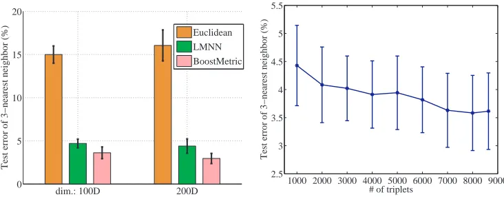
4.3.1 EXPERIMENT ON THECALTECH-101 DATASET
dim.: 100D 200D 0
5 10 15 20
Test error of 3−nearest neighbor (%)
Euclidean LMNN BoostMetric
1000 2000 3000 4000 5000 6000 7000 8000 9000 2.5
3 3.5 4 4.5 5 5.5
# of triplets
Test error of 3−nearest neighbor (%)
Figure 4: Test error (3-nearest neighbor) of BOOSTMETRIC on the Motorbikes versus Airplanes
data sets. The second plot shows the test error against the number of training triplets with a 100-word codebook.
Motorbikes versus Airplanes This experiment discriminates the images of a motorbike from
those of an airplane. In each of the 10 pairs of training/test subsets, there are 959 training images and 639 test images. Two visual codebooks of size 100 and 200 are used, respectively. With the
resulting histograms, the proposed BOOSTMETRICand the LMNN are learned on a training subset
and evaluated on the corresponding test subset. Their averaged classification error rates are
com-pared in Figure 4 (left). For both visual codebooks, the proposed BOOSTMETRICachieves lower
error rates than the LMNN and the Euclidean distance, demonstrating its superior performance. We also apply a linear SVM classifier with its regularization parameter carefully tuned by 5-fold cross-validation. Its error rates are 3.87%±0.69% and 3.00%±0.72% on the two visual code-books, respectively. In contrast, a 3NN with BOOSTMETRIC has error rates 3.63%±0.68% and
2.96%±0.59%. Hence, the performance of the proposed BOOSTMETRIC is comparable to the
state-of-the-art SVM classifier. Also, Figure 4 (right) plots the test error of the BOOSTMETRIC against the number of triplets for training. The general trend is that more triplets lead to smaller errors.
Faces versus Background-Google This experiment uses the two object classes as a retrieval
problem. The target of retrieval is face images. The images in the class of Background-Google are
randomly collected from the Internet and they represent the non-target class. BOOSTMETRIC is
5 10 15 20 0.3
0.4 0.5 0.6 0.7 0.8 0.9
rank
retrieval accuracy
input dim. 100
Euclidean LMNN BoostMetric
Figure 5: Retrieval accuracy of distance metric learning algorithms on the Faces versus Backgr-ound-Google data set. Error bars show the standard deviation.
4.3.2 EXPERIMENT ON THEMSRC DATASET
The 240 images of the MSRC database are randomly halved into 10 groups of training and test sets. Given a set of training images, the task is to predict the class label for each of the pre-segmented regions in a test image. We follow the work in Winn et al. (2005) to extract features and conduct experiments. Specifically, each image is converted from the RGB color space to the CIE Lab color space. First, three Gaussian low-pass filters are applied to the L, a, and b channels, respectively. The standard deviationσof the filters are set to 1, 2, and 4, respectively, and the filter size is defined as 4σ. This step produces 9 filter responses for each pixel in an image. Second, three Laplacian of Gaussian (LoG) filters are applied to the L channel only, with σ=1,2,4,8 and the filter size of 4σ. This step gives rise to 4 filter responses for each pixel. Lastly, the first derivatives of the Gaussian filter withσ=2,4 are computed from the L channel along the row and column directions, respectively. This results in 4 more filter responses. After applying this set of filter banks, each pixel is represented by a 17-dimensional feature vectors. All the feature vectors from a training set are clustered using the k-means clustering with a Mahalanobis distance.5 By setting k to 2000, a visual codebook of 2000 visual words is obtained. We implement the word-merging approach in Winn et al. (2005) and obtain a compact and discriminative codebook of 300 visual words. Each pre-segmented object region is then represented as a 300-dimensional histogram.
The proposed BOOSTMETRICis compared with the LMNN algorithm as follows. With 10
near-est neighbors information, about 20,000 triplets are constructed and used to train the BOOSTMET -RIC. To ensure convergence, the maximum number of iterations is set as 5000 in the optimization of
training BOOSTMETRIC. The training of LMNN follows the default setting. kNN classifiers with
the two learned Mahalanobis distances and the Euclidean distance are applied to each training and test group to categorize an object region. The categorization error rate on each test group is summa-rized in Table 3. As expected, both learned Mahalanobis distances achieve superior categorization
group index Euclidean LMNN BOOSTMETRIC
1 9.19 6.71 4.59
2 5.78 3.97 3.25
3 6.69 2.97 2.60
4 5.54 3.69 4.43
5 6.52 5.80 4.35
6 7.30 4.01 3.28
7 7.75 2.21 2.58
8 7.20 4.17 4.55
9 6.13 3.07 4.21
10 8.42 5.13 5.86
average: 7.05 4.17 3.97
standard devision: 1.16 1.37 1.03
Table 3: Comparison of the categorization performance.
Figure 6: Four generated triplets based on the pairwise information provided by the LFW data set. For the three images in each triplet, the first two belong to the same individual and the third one is a different individual.
performance to the Euclidean distance. Moreover, the proposed BOOSTMETRIC achieves better
performance than the LMNN, as indicated by its lower average categorization error rate and the
smaller standard deviation. Also, the kNN classifier using the proposed BOOSTMETRICachieves
comparable or even higher categorization performance than those reported in Winn et al. (2005).
Besides the categorization performance, we compare the computational efficiency of the BOOST
-METRICand the LMNN in learning a Mahalanobis distance. The computational time result is based on the Matlab codes for both methods. In this experiment, the average time cost by the BOOSTMET -RICfor learning the Mahalanobis distance is 3.98 hours, whereas the LMNN takes about 8.06 hours
to complete this process. Hence, the proposed BOOSTMETRIChas a shorter training process than
the LMNN method. This again demonstrates the computational advantage of the BOOSTMETRIC
over the LMNN method.
4.4 Unconstrained Face Recognition
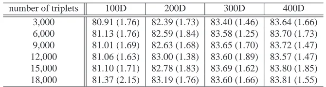
number of triplets 100D 200D 300D 400D 3,000 80.91 (1.76) 82.39 (1.73) 83.40 (1.46) 83.64 (1.66) 6,000 81.13 (1.76) 82.59 (1.84) 83.58 (1.25) 83.70 (1.73) 9,000 81.01 (1.69) 82.63 (1.68) 83.65 (1.70) 83.72 (1.47) 12,000 81.06 (1.63) 83.00 (1.38) 83.60 (1.89) 83.57 (1.47) 15,000 81.10 (1.71) 82.78 (1.83) 83.69 (1.62) 83.80 (1.85) 18,000 81.37 (2.15) 83.19 (1.76) 83.60 (1.66) 83.81 (1.55)
Table 4: Comparison of the face recognition accuracy (%) of our proposed BOOSTMETRICon the
LFW data set by varying the PCA dimensionality and the number of triplets for each fold.
This is a data set of unconstrained face images, which has a large range of variations seen in real world, including 13,233 images of 5,749 people collected from news articles on Internet. The face recognition task here is pair matching—given two face images, to determine if these two images are of the same individual. So we classify unseen pairs to determine whether each image in the pair indicates the same individual or not, by applying MkNN of Guillaumin et al. (2009) instead of kNN. Features of face images are extracted by computing 3-scale, 128-dimensional SIFT descriptors (Lowe, 2004), which center on 9 points of facial features extracted by a facial feature descriptor, same as described in Guillaumin et al. (2009). PCA is then performed on the SIFT vectors to reduce the dimension to between 100 and 400.
Simple recognition systems with a single descriptor Table 4 shows our BOOSTMETRIC’s
per-formance by varying PCA dimensionality and the number of triplets. Increasing the number of training triplets gives slight improvement of recognition accuracy. The dimension after PCA has more impact on the final accuracy for this task.
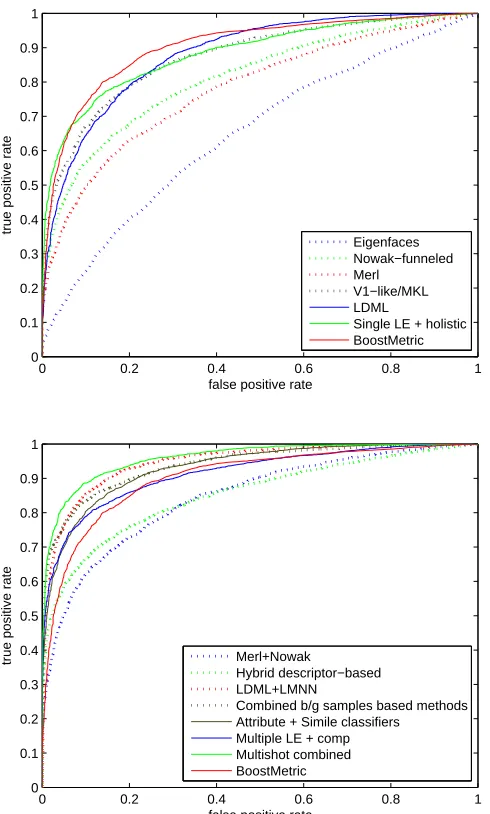
In Figure 7, we have drawn ROC curves of other algorithms for face recognition. To obtain our ROC curve, MkNN has moved the threshold value across the distributions of match and mismatch similarity scores. Figure 7 (a) shows methods that use a single descriptor and a single classifier only. As can be seen, our system using BOOSTMETRICoutperforms all the others in the literature with a very small computational cost.
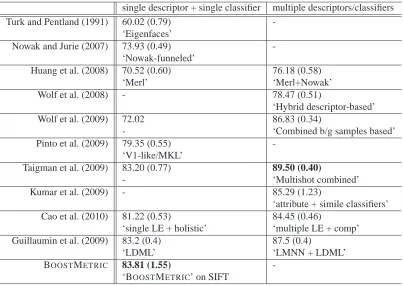
Complex recognition systems with one or more descriptors Figure 7 (b) plots the performance
of more complicated recognition systems that use hybrid descriptors or combination of classifiers.
See Table 5 for details. We can see that the performance of our BOOSTMETRIC is close to the
state-of-the-art.
In particular, BOOSTMETRICoutperforms the method of Guillaumin et al. (2009), which has a similar pipeline but uses LMNN for learning a metric. This comparison also confirms the impor-tance of learning an appropriate metric for vision problems.
5. Conclusion
We have presented a new algorithm, BOOSTMETRIC, to learn a positive semidefinite metric using
boosting techniques. We have generalized AdaBoost in the sense that the weak learner of BOOST
0 0.2 0.4 0.6 0.8 1 0
0.1 0.2 0.3 0.4 0.5 0.6 0.7 0.8 0.9 1
false positive rate
true positive rate
Eigenfaces Nowak−funneled Merl
V1−like/MKL LDML
Single LE + holistic BoostMetric
0 0.2 0.4 0.6 0.8 1 0
0.1 0.2 0.3 0.4 0.5 0.6 0.7 0.8 0.9 1
false positive rate true positive rate Merl+Nowak
Hybrid descriptor−based LDML+LMNN
Combined b/g samples based methods Attribute + Simile classifiers
Multiple LE + comp Multishot combined BoostMetric
Figure 7: (top) ROC Curves that use a single descriptor and a single classifier, (bottom) ROC curves that use hybrid descriptors are plotted. Our BOOSTMETRIC with a single classifier is also plotted. Each point on the curves is the average over the 10 folds of rates for a fixed threshold.
We also want to learn a metric using BOOSTMETRIC in the semi-supervised, and multi-task
learning setting. It has been shown in Weinberger and Saul (2009) that the classification
perfor-mance can be improved by learning multiple local metrics. We will extend BOOSTMETRICto learn
multiple metrics. Finally, we will explore to generalize BOOSTMETRIC for solving more general
single descriptor + single classifier multiple descriptors/classifiers Turk and Pentland (1991) 60.02 (0.79)
-‘Eigenfaces’
Nowak and Jurie (2007) 73.93 (0.49) -‘Nowak-funneled’
Huang et al. (2008) 70.52 (0.60) 76.18 (0.58)
‘Merl’ ‘Merl+Nowak’
Wolf et al. (2008) - 78.47 (0.51)
‘Hybrid descriptor-based’
Wolf et al. (2009) 72.02 86.83 (0.34)
- ‘Combined b/g samples based’
Pinto et al. (2009) 79.35 (0.55) -‘V1-like/MKL’
Taigman et al. (2009) 83.20 (0.77) 89.50 (0.40)
- ‘Multishot combined’
Kumar et al. (2009) - 85.29 (1.23)
‘attribute + simile classifiers’ Cao et al. (2010) 81.22 (0.53) 84.45 (0.46)
‘single LE + holistic’ ‘multiple LE + comp’ Guillaumin et al. (2009) 83.2 (0.4) 87.5 (0.4)
‘LDML’ ‘LMNN + LDML’
BOOSTMETRIC 83.81 (1.55)
-‘BOOSTMETRIC’ on SIFT
Table 5: Test accuracy in percentage (mean and standard deviation) on the LFW data set. ROC curve labels in Figure 7 are described here with details.
References
A. Bar-Hillel, T. Hertz, N. Shental, and D. Weinshall. Learning a Mahalanobis metric from equiva-lence constraints. J. Machine Learning Research, 6:937–965, 2005.
O. Boiman, E. Shechtman, and M. Irani. In defense of nearest-neighbor based image classification. In Proc. IEEE Int’l Conf. Computer Vision and Pattern Recognition, 2008.
B. Borchers. CSDP, a C library for semidefinite programming. Optimization Methods and Software, 11(1):613–623, 1999.
S. Boyd and L. Vandenberghe. Convex Optimization. Cambridge University Press, 2004.
Z. Cao, Q. Yin, X. Tang, and J. Sun. Face recognition with learning-based descriptor. In Proc. IEEE
Int’l Conf. Computer Vision and Pattern Recognition, 2010.
G. B. Dantzig and P. Wolfe. Decomposition principle for linear programs. Operation Research, 8 (1):101–111, 1960.
J. V. Davis, B. Kulis, P. Jain, S. Sra, and I. S. Dhillon. Information-theoretic metric learning. In