Adv. Radio Sci., 4, 135–141, 2006 www.adv-radio-sci.net/4/135/2006/ © Author(s) 2006. This work is licensed under a Creative Commons License.
Advances in
Radio Science
Feature selection with acquisition cost for optimizing
sensor system design
K. Iswandy and A. Koenig
Institute of Integrated Sensor Systems, University of Kaiserslautern, Erwin-Schroedinger-Str., 67663 Kaiserslautern, Germany
Abstract. Selection of variables from large sets of
measure-ments is a common problem of data analysis and signal pro-cessing in many disciplines. In engineering and sensor tech-nology the design of recognition systems can be optimized by judicious choice of subsets of relevant features. In par-ticular, the effort required for signal processing and sensor registration can be considerably reduced by efficient feature selection. However, the current approaches in majority only consider the contribution of features or measurements to the classification ability of the system. The associated cost in terms of computation effort, the required electronics, and power dissipation is not explicitly in consideration. This pa-per proposes a multi-objective extension of feature selection including acquisition cost and employing and comparing two evolutionary optimization methods. The genetic and particle swarm algorithms and the results achieved with selected data sets will be presented. The results show, that particle swarm algorithm can select best features with lower cost and achieve more competitive results with regard to convergence time and classification accuracy than genetic algorithm.
1 Introduction
In many real-world applications such as pattern recognition and machine learning, the tasks of object detection often deal with large number of measurements or high dimensional data sets. In particular, in engineering and sensor technology, these large number of measurements or variables (here called features) usually contain some irrelevant and/or redundant features (Langley, 1996), which can degrade the reliability of system performance with regard to the accuracy of the clas-sification. Therefore, the unnecessary features must be elim-inated by using methods of dimensionality reduction. One Correspondence to: K. Iswandy
of the dimensionality reduction methods is feature selection, which is focused in this paper for optimizing sensor system design, applying to select a feature subset with the best per-formance (Jain and Zongker, 1997). Furthermore, the ac-quisition cost is an important issue (Pacl´ık et al., 2002) in some applications, for example, medical diagnosis (time and price), electronics (power dissipation), texture segmentation (computational effort), etc. The current approaches in ma-jority only consider the contribution of features or measure-ments to the classification ability of the system. The inten-tion of associated cost is to preserve the quality with regard to classification with least expensive features. The aims of this paper are to propose a multi-objective extension of feature selection and acquisition cost employing two evolutionary computation methods, i.e. genetic algorithm (GA) and par-ticle swarm optimization (PSO), in an optimization scheme and to compare the results between GA and PSO with regard to the reliability (classification accuracy) and the speed (com-putation and convergency). Figure 1 shows the process of optimization of sensor system design, where the applications of recognition system often use multiple sensors for object measurement. The sensors produce signals as measurement results and these signals, which are sampled in the certain time interval, are represented as array vectors. The array vec-tors will be processed by some feature computation methods (e.g. mean, standard deviation or variance, histogram, wave amplitude and duration, etc.) to obtain concatenated feature vectors. These feature vectors will be optimized with subset of relevant features associated with acquisition cost and the sensorial effort will be saved due to efficient selection. In the next section the feature selection is briefly presented.
2 Brief survey of feature selection
Feature selection is a method to find minimum feature subset giving optimum discrimination between two or more
136 K. Iswandy and A. Koenig: Feature selection with acquisition cost
2
K. Iswandy and A. Koenig: Feature Selection with Acquisition Cost
Mean, µ
Std, ı
etc. x1 x2 . . xn t y(t) t Sensor 1 Sensor 1 Sensor 2 Sensor 2 Sensor 3 Sensor 3 Sensor K Sensor K Feature Computation 1 Feature Computation 1 Feature Computation 2 Feature Computation 2 Feature Computation M Feature Computation M k1 k2 kM D im e n s io n a lit y R e d u c tio n (AFS) C la s s ifi e r S tr u c tu re to A c tu a to r kdr Elimination according to DR
Elimination according to DR
Fig. 1. The process of sensor system design for recognition system
with optimizing structure.
Sensor Raw Feature
Computation y = Asx Classifier
Train/Test Assessment and
Modification of As
classification result (J)
Fig. 2. The wrapper approach to automatic feature selection.
dependently of the learning algorithm or classifier as shown
in Fig. 2 and (2) filter approach that is performed
indepen-dently of the classifier as shown in Fig. 3. In general, the
wrapper method provides features that lead to more
accu-rate classification than that of the filter method. However,
the filter method executes many times faster than wrapper
method, and therefore stands a much better chance of scaling
to datasets with a large number of features than the wrapper
does (Mao, 2002).
Moreover, feature selection can be viewed as a heuristic
search, where each state in the search space represents a
par-ticular subset of the available features. In all but the
splest cases, an exhaustive search of the state space is
im-practical for even moderate number of features (Jain et al.,
2000), since it is also known as a combinatorial
optimiza-tion problem. However, exhaustive search can be applied
well for a small number of features.
Several search
ap-proaches have been applied to this problem, ranging from
simple greedy approaches such as sequential forward
selec-tion (SFS), sequential backward selecselec-tion (SBS), and
com-bination SFS and SBS called floating search (Siedlecki and
Sklansky, 1988). The more powerful approach for
optimiza-tion strategies have been proposed such as genetic algorithm
(Siedlecki and Sklansky, 1989) and recently binary particle
swarm (Agrafiotis and Cedeno, 2002).
The AFS is a special case of a more general technique
known as feature weighting (Aha, 1998; Koenig, 2000) and
a linear mapping based on the selection matrix
A
Swith
Sensor Raw Feature
Computation y = Asx Classifier
Train/Test Assessment and
Modification of As
classification result J
Fig. 3. The filter approach to automatic feature selection.
Y
=
A
SX
, where
X
is a set of
d
features.
A
S=
c1
0 0
· · ·
0
0
c2
0
· · ·
0
· · · ·
0 0
· · ·
c
d−10
0 0 0
· · ·
c
d
In feature weighting, each feature is associated with weight
value that indicates the contribution of that feature in the
learning algorithm. According to the feature weighting, there
are two categories: (1) feature weighting and (2) feature
selection. For feature weighting, the weighting values are
arbitrary real number and usually confined to the interval
c
i∈
[0
,
1]
. In feature selection, a weight can either be 1
or 0 to indicate whether the feature is used in the model or
not (switch variables). In this paper, we consider only feature
selection with using filter approach.
The optimum discrimination according to subset features
is determined by an objective function
J
. In the filter model,
there are several objective functions for feature
assess-ment measures such as simple parametric overlap measure,
nonparametric overlap measure, nonparametric compactness
measure, nonparametric separability measure (Koenig, 2001;
Koenig and Gratz, 2005), etc. In this paper, a supervised
non-parametric overlap measure (NPOM) is applied as one
crite-rion for feature space assessment with regard to class regions
overlap. NPOM is inspired by nearest-neighbor concepts.
This normalized measure gives values close to one for
non-overlapping class regions and decreases towards zero
pro-portional to increasingly overlapping of class regions. The
NPOM, also denoted as
Q
ovin the following, is expressed as
Q
ov=
1
L
LX
c=11
N
c NcX
j=1P
ki=1
q
N Nji+
P
ki=1
n
i2
×
P
ki=1n
i(1)
with
n
i= 1
−
d
N Njid
N Njkand
q
N Nji=
½
n
iif
ω
j=
ω
i−
n
iif
ω
j6
=
ω
iwhere
d
N Njiis the Euclidean distance between the regarded
pattern and one of its nearest neighbor and
ω
denotes the
class affiliation of the regarding pattern.
Fig. 1. The process of sensor system design for recognition system with optimizing structure.
ously defined groups of objects. This feature selection is an iterative algorithm (also called automatic feature selection or AFS). The AFS can be divided into two groups (Kohavi and John, 1998):
(1) wrapper approach that is performed dependently of the learning algorithm or classifier as shown in Fig. 2 and (2) filter approach that is performed independently of the classifier as shown in Fig. 3.
In general, the wrapper method provides features that lead to more accurate classification than that of the filter method. However, the filter method executes many times faster than wrapper method, and therefore stands a much better chance of scaling to datasets with a large number of features than the wrapper does (Mao, 2002).
Moreover, feature selection can be viewed as a heuristic search, where each state in the search space represents a par-ticular subset of the available features. In all but the splest cases, an exhaustive search of the state space is im-practical for even moderate number of features (Jain et al., 2000), since it is also known as a combinatorial optimiza-tion problem. However, exhaustive search can be applied well for a small number of features. Several search ap-proaches have been applied to this problem, ranging from simple greedy approaches such as sequential forward selec-tion (SFS), sequential backward selecselec-tion (SBS), and com-bination SFS and SBS called floating search (Siedlecki and Sklansky, 1988). The more powerful approach for optimiza-tion strategies have been proposed such as genetic algorithm (Siedlecki and Sklansky, 1989) and recently binary particle swarm (Agrafiotis and Cedeno, 2002).
The AFS is a special case of a more general technique known as feature weighting (Aha, 1998; Koenig, 2000) and a linear mapping based on the selection matrix AS with
Mean, µ
Std, ı
etc. x1 x2 . . xn t y(t) t Sensor 1 Sensor 1 Sensor 2 Sensor 2 Sensor 3 Sensor 3 Sensor K Sensor K Feature Computation 1 Feature Computation 1 Feature Computation 2 Feature Computation 2 Feature Computation M Feature Computation M k1 k2 kM D im e n s io n a lit y R e d u c tio n (AFS) C la s s ifi e r S tr u c tu re to A c tu a to r kdr Elimination according to DR
Elimination according to DR
Fig. 1. The process of sensor system design for recognition system
with optimizing structure.
Sensor Raw Feature
Computation y = Asx Train/TestClassifier
Assessment and
Modification of As
classification result (J)
Fig. 2. The wrapper approach to automatic feature selection.
dependently of the learning algorithm or classifier as shown
in Fig. 2 and (2) filter approach that is performed
indepen-dently of the classifier as shown in Fig. 3. In general, the
wrapper method provides features that lead to more
accu-rate classification than that of the filter method. However,
the filter method executes many times faster than wrapper
method, and therefore stands a much better chance of scaling
to datasets with a large number of features than the wrapper
does (Mao, 2002).
Moreover, feature selection can be viewed as a heuristic
search, where each state in the search space represents a
par-ticular subset of the available features. In all but the
splest cases, an exhaustive search of the state space is
im-practical for even moderate number of features (Jain et al.,
2000), since it is also known as a combinatorial
optimiza-tion problem. However, exhaustive search can be applied
well for a small number of features.
Several search
ap-proaches have been applied to this problem, ranging from
simple greedy approaches such as sequential forward
selec-tion (SFS), sequential backward selecselec-tion (SBS), and
com-bination SFS and SBS called floating search (Siedlecki and
Sklansky, 1988). The more powerful approach for
optimiza-tion strategies have been proposed such as genetic algorithm
(Siedlecki and Sklansky, 1989) and recently binary particle
swarm (Agrafiotis and Cedeno, 2002).
The AFS is a special case of a more general technique
known as feature weighting (Aha, 1998; Koenig, 2000) and
a linear mapping based on the selection matrix
A
Swith
Sensor Raw Feature
Computation y = Asx
Classifier Train/Test Assessment and
Modification of As
classification result J
Fig. 3. The filter approach to automatic feature selection.
Y
=
A
SX
, where
X
is a set of
d
features.
A
S=
c1
0 0
· · ·
0
0
c2
0
· · ·
0
· · · ·
0 0
· · ·
c
d−10
0 0 0
· · ·
c
d
In feature weighting, each feature is associated with weight
value that indicates the contribution of that feature in the
learning algorithm. According to the feature weighting, there
are two categories: (1) feature weighting and (2) feature
selection. For feature weighting, the weighting values are
arbitrary real number and usually confined to the interval
c
i∈
[0
,
1]
. In feature selection, a weight can either be 1
or 0 to indicate whether the feature is used in the model or
not (switch variables). In this paper, we consider only feature
selection with using filter approach.
The optimum discrimination according to subset features
is determined by an objective function
J
. In the filter model,
there are several objective functions for feature
assess-ment measures such as simple parametric overlap measure,
nonparametric overlap measure, nonparametric compactness
measure, nonparametric separability measure (Koenig, 2001;
Koenig and Gratz, 2005), etc. In this paper, a supervised
non-parametric overlap measure (NPOM) is applied as one
crite-rion for feature space assessment with regard to class regions
overlap. NPOM is inspired by nearest-neighbor concepts.
This normalized measure gives values close to one for
non-overlapping class regions and decreases towards zero
pro-portional to increasingly overlapping of class regions. The
NPOM, also denoted as
Q
ovin the following, is expressed as
Q
ov=
1
L
LX
c=11
N
c NcX
j=1P
ki=1
q
N Nji+
P
ki=1
n
i2
×
P
ki=1n
i(1)
with
n
i= 1
−
d
N Njid
N Njkand
q
N Nji=
½
n
iif
ω
j=
ω
i−
n
iif
ω
j6
=
ω
iwhere
d
N Njiis the Euclidean distance between the regarded
pattern and one of its nearest neighbor and
ω
denotes the
class affiliation of the regarding pattern.
Fig. 2. The wrapper approach to automatic feature selection.
2
K. Iswandy and A. Koenig: Feature Selection with Acquisition Cost
Mean, µ
Std, ı
etc. x1 x2 . . xn t y(t) t Sensor 1 Sensor 1 Sensor 2 Sensor 2 Sensor 3 Sensor 3 Sensor K Sensor K Feature Computation 1 Feature Computation 1 Feature Computation 2 Feature Computation 2 Feature Computation M Feature Computation M k1 k2 kM D im e n s io n a lit y R e d u c tio n (AFS) C la s s ifi e r S tr u c tu re to A c tu a to r kdr Elimination according to DR
Elimination according to DR
Fig. 1. The process of sensor system design for recognition system
with optimizing structure.
Sensor Raw Feature
Computation y = Asx
Classifier Train/Test Assessment and
Modification of As
classification result (J)
Fig. 2. The wrapper approach to automatic feature selection.
dependently of the learning algorithm or classifier as shown
in Fig. 2 and (2) filter approach that is performed
indepen-dently of the classifier as shown in Fig. 3. In general, the
wrapper method provides features that lead to more
accu-rate classification than that of the filter method. However,
the filter method executes many times faster than wrapper
method, and therefore stands a much better chance of scaling
to datasets with a large number of features than the wrapper
does (Mao, 2002).
Moreover, feature selection can be viewed as a heuristic
search, where each state in the search space represents a
par-ticular subset of the available features. In all but the
splest cases, an exhaustive search of the state space is
im-practical for even moderate number of features (Jain et al.,
2000), since it is also known as a combinatorial
optimiza-tion problem. However, exhaustive search can be applied
well for a small number of features.
Several search
ap-proaches have been applied to this problem, ranging from
simple greedy approaches such as sequential forward
selec-tion (SFS), sequential backward selecselec-tion (SBS), and
com-bination SFS and SBS called floating search (Siedlecki and
Sklansky, 1988). The more powerful approach for
optimiza-tion strategies have been proposed such as genetic algorithm
(Siedlecki and Sklansky, 1989) and recently binary particle
swarm (Agrafiotis and Cedeno, 2002).
The AFS is a special case of a more general technique
known as feature weighting (Aha, 1998; Koenig, 2000) and
a linear mapping based on the selection matrix
A
Swith
Sensor Raw Feature
Computation y = Asx Classifier
Train/Test Assessment and
Modification of As
classification result J
Fig. 3. The filter approach to automatic feature selection.
Y
=
A
SX
, where
X
is a set of
d
features.
A
S=
c1
0 0
· · ·
0
0
c2
0
· · ·
0
· · · ·
0 0
· · ·
c
d−10
0 0 0
· · ·
c
d
In feature weighting, each feature is associated with weight
value that indicates the contribution of that feature in the
learning algorithm. According to the feature weighting, there
are two categories: (1) feature weighting and (2) feature
selection. For feature weighting, the weighting values are
arbitrary real number and usually confined to the interval
c
i∈
[0
,
1]
. In feature selection, a weight can either be 1
or 0 to indicate whether the feature is used in the model or
not (switch variables). In this paper, we consider only feature
selection with using filter approach.
The optimum discrimination according to subset features
is determined by an objective function
J
. In the filter model,
there are several objective functions for feature
assess-ment measures such as simple parametric overlap measure,
nonparametric overlap measure, nonparametric compactness
measure, nonparametric separability measure (Koenig, 2001;
Koenig and Gratz, 2005), etc. In this paper, a supervised
non-parametric overlap measure (NPOM) is applied as one
crite-rion for feature space assessment with regard to class regions
overlap. NPOM is inspired by nearest-neighbor concepts.
This normalized measure gives values close to one for
non-overlapping class regions and decreases towards zero
pro-portional to increasingly overlapping of class regions. The
NPOM, also denoted as
Q
ovin the following, is expressed as
Q
ov=
1
L
LX
c=11
N
c NcX
j=1P
ki=1
q
N Nji+
P
ki=1
n
i2
×
P
ki=1n
i(1)
with
n
i= 1
−
d
N Njid
N Njkand
q
N Nji=
½
n
iif
ω
j=
ω
i−
n
iif
ω
j6
=
ω
iwhere
d
N Njiis the Euclidean distance between the regarded
pattern and one of its nearest neighbor and
ω
denotes the
class affiliation of the regarding pattern.
Fig. 3. The filter approach to automatic feature selection.
Y =ASX, whereXis a set ofdfeatures.
AS=
c1 0 0 · · · 0
0 c2 0 · · · 0
· · · ·
0 0 · · ·cd−1 0
0 0 0 · · · cd
In feature weighting, each feature is associated with weight value that indicates the contribution of that feature in the learning algorithm. According to the feature weighting, there are two categories: (1) feature weighting and (2) feature selection. For feature weighting, the weighting values are arbitrary real number and usually confined to the interval ci ∈ [0,1]. In feature selection, a weight can either be 1 or 0 to indicate whether the feature is used in the model or not (switch variables). In this paper, we consider only feature selection with using filter approach.
The optimum discrimination according to subset features is determined by an objective functionJ. In the filter model, there are several objective functions for feature assess-ment measures such as simple parametric overlap measure, nonparametric overlap measure, nonparametric compactness measure, nonparametric separability measure (Koenig, 2001; Koenig and Gratz, 2005), etc. In this paper, a supervised non-parametric overlap measure (NPOM) is applied as one crite-rion for feature space assessment with regard to class regions overlap. NPOM is inspired by nearest-neighbor concepts. This normalized measure gives values close to one for non-overlapping class regions and decreases towards zero pro-portional to increasingly overlapping of class regions. The NPOM, also denoted asQovin the following, is expressed as
Qov= 1 L L X c=1 1 Nc Nc X j=1 Pk
i=1qN Nj i+ Pk
i=1ni 2×Pk
i=1ni
(1)
K. Iswandy and A. Koenig: Feature selection with acquisition cost 137
K. Iswandy and A. Koenig: Feature Selection with Acquisition Cost
3
3
Feature Selection with Acquisition Cost
In many applications, the measurement or computation
pro-cess of object features is always associated with certain cost.
The cost can be price of medical diagnosis, power
dissipa-tion in electronics, time or computadissipa-tion complexity, etc. The
usage of feature selection method in majority only consider
the contribution of features or measurements to the
classifi-cation ability of the system. The accumulation of acquisition
cost within automatic feature selection (AFSC) is still rarely
investigated. With regard to including acquisition cost our
work is similar to Pacl´ık et al. (2002) and Yang and Honavar
(1998). However, our approach is more general and employs
advanced optimization techniques from evolutionary
compu-tation.
To optimize two or more objective functions, the
multi-objectives optimization approaches will be used. In
partic-ular, the weighted aggregation method is applied in this
pa-per, since this method is the simplest one (Zitzler and Thiele,
1999). According to this approach, all the objectives are
summed to a weighted combination
F
=
P
pi=1ω
if
i(
x
)
,
where the weights are non-negative weights. It is usually
assumed that
P
pi=1ω
i= 1
. In this paper, we used one
fea-ture assessment function (NPOM) and a cost function. The
accumulative expression is
K
=
w
1×
Q
ov+
w
2×
µ
1
−
C
SC
T
(2)
where
w
i: weight of objective functions,
C
S: sum of selected
features cost, and
C
T: sum of total feature cost. The weight
values used in all of our experiments were 0.6 and 0.4.
4
Optimization Methods
4.1
Genetic Algorithm
Genetic algorithm or GA is a class of optimization
pro-cedures inspired by the biology mechanisms of
reproduc-tion. GA operates iteratively on a population of structures,
each one of which represents a candidate solution to the
problem at hand, properly encoded as a string of symbols
(e.g., binary). A random generated set of such strings forms
the initial population from which the GA starts its search.
Three basic genetic operators guide this search, i.e.,
selec-tion, crossover, and mutation (Goldberg, 1989). The
candi-date solution or chromosome is a bit string whose length is
determined by the number of features. The fitness function is
used according to Eq. (1) for optimizing the AFS or Eq. (2)
for optimizing the AFSC. The main algorithm is given
be-low:
1. Initialization: Generate an initial population using a
random mechanism. Denote the population as
P
i=
{
p
1, ...,
p
N}
, where N is the population size and
p
=
{
f
1, ...,
f
n}
, where n is feature size.
P1
P2
Ofs1
Ofs2
Random
1
0 1 1 0 0 0 1 1 1
1
0 0 0 0 0 1 0 1 0
1
0 1
1 0 0 0 1 1 1
1 0
0 0 0 0 1 0
0
1
Fig. 4. One-point crossover.
P
Random Random
Ofs 1
0 1 0 0 0 0 1 1 1
1
0 0 0 0 0 1 1 1 0
Fig. 5. Mutation.
2. Selection: Roulette wheel selection is used to select
can-didates into the mating pool and the selection
probabil-ity of each individual is based on its proportional
fit-ness value. Selected candidates represent an
interme-diate population,
P
s, that has same size with current
population.
3. Crossover: Here, one-point crossover takes place for
search process and information exchange between two
chromosomes from parent population. The parent
chro-mosomes are split at a common point chosen
ran-domly and the resulting sub-chromosomes are swapped
(Fig. 4). This generates a next intermediate
popula-tion
P
rfrom
P
s, where each two individuals take the
crossover process and produce two offsprings.
The
crossover probability used in all of our experiments was
0.95.
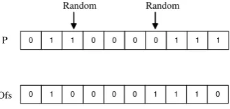
4. Mutation: After the crossover process, the mutation
generates the next intermediate population
P
m. Each
individual from
P
rproduces an offspring. Here, we use
the traditional mutation operator which flips a specific
bit with a very low probability (Fig. 5). The mutation
probability used in all of our experiments was 0.01.
5. Reproduction: Offsprings from
P
mwill be selected
into the next generation. The best
10%
individuals of
parent will be taken and competed with offsprings based
on their fitness values. If the best parent is better than
the offspring, then the best parent will be reproduced
for next generation
P
i+1and otherwise, they will be
discarded.
6. Termination condition: The termination condition of
this algorithm is referred to a pre-specified number of
generation and criterion of fitness value. The algorithm
Fig. 4. One-point crossover.
with ni =1−
dN Nj i
dN Nj k
and qN Nj i =
ni ifωj =ωi
−ni ifωj 6=ωi
wheredN Nj i is the Euclidean distance between the regarded
pattern and one of its nearest neighbor andω denotes the class affiliation of the regarding pattern.
3 Feature selection with acquisition cost
In many applications, the measurement or computation pro-cess of object features is always associated with certain cost. The cost can be price of medical diagnosis, power dissipa-tion in electronics, time or computadissipa-tion complexity, etc. The usage of feature selection method in majority only consider the contribution of features or measurements to the classifi-cation ability of the system. The accumulation of acquisition cost within automatic feature selection (AFSC) is still rarely investigated. With regard to including acquisition cost our work is similar to Pacl´ık et al. (2002) and Yang and Honavar (1998). However, our approach is more general and em-ploys advanced optimization techniques from evolutionary computation.
To optimize two or more objective functions, the multi-objectives optimization approaches will be used. In par-ticular, the weighted aggregation method is applied in this paper, since this method is the simplest one (Zitzler and Thiele, 1999). According to this approach, all the objectives are summed to a weighted combinationF=Pp
i=1ωifi(x),
where the weights are non-negative weights. It is usually as-sumed thatPp
i=1ωi=1. In this paper, we used one feature
assessment function (NPOM) and a cost function. The accu-mulative expression is
K=w1×Qov+w2×
1−CS
CT
(2)
K. Iswandy and A. Koenig: Feature Selection with Acquisition Cost
3
3
Feature Selection with Acquisition Cost
In many applications, the measurement or computation
pro-cess of object features is always associated with certain cost.
The cost can be price of medical diagnosis, power
dissipa-tion in electronics, time or computadissipa-tion complexity, etc. The
usage of feature selection method in majority only consider
the contribution of features or measurements to the
classifi-cation ability of the system. The accumulation of acquisition
cost within automatic feature selection (AFSC) is still rarely
investigated. With regard to including acquisition cost our
work is similar to Pacl´ık et al. (2002) and Yang and Honavar
(1998). However, our approach is more general and employs
advanced optimization techniques from evolutionary
compu-tation.
To optimize two or more objective functions, the
multi-objectives optimization approaches will be used. In
partic-ular, the weighted aggregation method is applied in this
pa-per, since this method is the simplest one (Zitzler and Thiele,
1999). According to this approach, all the objectives are
summed to a weighted combination
F
=
P
pi=1ω
if
i(
x
)
,
where the weights are non-negative weights. It is usually
assumed that
P
pi=1ω
i= 1
. In this paper, we used one
fea-ture assessment function (NPOM) and a cost function. The
accumulative expression is
K
=
w
1×
Q
ov+
w
2×
µ
1
−
C
SC
T
(2)
where
w
i: weight of objective functions,
C
S: sum of selected
features cost, and
C
T: sum of total feature cost. The weight
values used in all of our experiments were 0.6 and 0.4.
4
Optimization Methods
4.1
Genetic Algorithm
Genetic algorithm or GA is a class of optimization
pro-cedures inspired by the biology mechanisms of
reproduc-tion. GA operates iteratively on a population of structures,
each one of which represents a candidate solution to the
problem at hand, properly encoded as a string of symbols
(e.g., binary). A random generated set of such strings forms
the initial population from which the GA starts its search.
Three basic genetic operators guide this search, i.e.,
selec-tion, crossover, and mutation (Goldberg, 1989). The
candi-date solution or chromosome is a bit string whose length is
determined by the number of features. The fitness function is
used according to Eq. (1) for optimizing the AFS or Eq. (2)
for optimizing the AFSC. The main algorithm is given
be-low:
1. Initialization: Generate an initial population using a
random mechanism. Denote the population as
P
i=
{
p
1, ...,
p
N}
, where N is the population size and
p
=
{
f
1, ...,
f
n}
, where n is feature size.
P1
P2
Ofs1
Ofs2
Random
1
0 1 1 0 0 0 1 1 1
1
0 0 0 0 0 1 0 1 0
1
0 1
1 0 0 0 1 1 1
1 0
0 0 0 0 1 0
0
1
Fig. 4. One-point crossover.
P
Random Random
Ofs 1
0 1 0 0 0 0 1 1 1
1
0 0 0 0 0 1 1 1 0
Fig. 5. Mutation.
2. Selection: Roulette wheel selection is used to select
can-didates into the mating pool and the selection
probabil-ity of each individual is based on its proportional
fit-ness value. Selected candidates represent an
interme-diate population,
P
s, that has same size with current
population.
3. Crossover: Here, one-point crossover takes place for
search process and information exchange between two
chromosomes from parent population. The parent
chro-mosomes are split at a common point chosen
ran-domly and the resulting sub-chromosomes are swapped
(Fig. 4). This generates a next intermediate
popula-tion
P
rfrom
P
s, where each two individuals take the
crossover process and produce two offsprings.
The
crossover probability used in all of our experiments was
0.95.
4. Mutation: After the crossover process, the mutation
generates the next intermediate population
P
m. Each
individual from
P
rproduces an offspring. Here, we use
the traditional mutation operator which flips a specific
bit with a very low probability (Fig. 5). The mutation
probability used in all of our experiments was 0.01.
5. Reproduction: Offsprings from
P
mwill be selected
into the next generation. The best
10%
individuals of
parent will be taken and competed with offsprings based
on their fitness values. If the best parent is better than
the offspring, then the best parent will be reproduced
for next generation
P
i+1and otherwise, they will be
discarded.
6. Termination condition: The termination condition of
this algorithm is referred to a pre-specified number of
generation and criterion of fitness value. The algorithm
Fig. 5. Mutation.
wherewi: weight of objective functions,CS: sum of selected features cost, andCT: sum of total feature cost. The weight values used in all of our experiments were 0.6 and 0.4.
4 Optimization methods
4.1 Genetic algorithm
Genetic algorithm or GA is a class of optimization proce-dures inspired by the biology mechanisms of reproduction. GA operates iteratively on a population of structures, each one of which represents a candidate solution to the problem at hand, properly encoded as a string of symbols (e.g. binary). A random generated set of such strings forms the initial pop-ulation from which the GA starts its search. Three basic ge-netic operators guide this search, i.e. selection, crossover, and mutation (Goldberg, 1989). The candidate solution or chro-mosome is a bit string whose length is determined by the number of features. The fitness function is used according to Eq. (1) for optimizing the AFS or Eq. (2) for optimizing the AFSC. The main algorithm is given below:
1. Initialization: Generate an initial population using a random mechanism. Denote the population as Pi= {p1, ...,pN}, where N is the population size and
p= {f1, ...,fn}, where n is feature size.
2. Selection: Roulette wheel selection is used to select can-didates into the mating pool and the selection probabil-ity of each individual is based on its proportional fit-ness value. Selected candidates represent an interme-diate population, Ps, that has same size with current population.
3. Crossover: Here, one-point crossover takes place for search process and information exchange between two chromosomes from parent population. The parent chro-mosomes are split at a common point chosen ran-domly and the resulting sub-chromosomes are swapped (Fig. 4). This generates a next intermediate popula-tionPr fromPs, where each two individuals take the crossover process and produce two offsprings. The crossover probability used in all of our experiments was 0.85.
4. Mutation: After the crossover process, the mutation generates the next intermediate populationPm. Each individual fromPrproduces an offspring. Here, we use the traditional mutation operator which flips a specific bit with a very low probability (Fig. 5). The mutation probability used in all of our experiments was 0.01. 5. Reproduction: Offsprings fromPmwill be selected into
the next generation. The best 10% individuals of par-ent will be taken and competed with offsprings based on their fitness values. If the best parent is better than the offspring, then the best parent will be reproduced for next generationPi+1 and otherwise, they will be
discarded.
6. Termination condition: The termination condition of this algorithm is referred to a pre-specified number of generation and criterion of fitness value. The algorithm will stop, if one of these two conditions are reached; otherwise go to step 2.
4.2 Binary particle swarm optimization
Particle swarm optimization (PSO) is a non-linear method which also is affiliated to evolutionary computation tech-niques. This method is a relatively new optimization paradigm introduced by Kennedy and Eberhart (1995). Parti-cle swarms explore the search space through a population of particles, which adapt by returning to previously successful regions. The particles then fly over the state space, remem-bering the best solution encountered. The fitness function is determined by an application-specific objective function (here, Eq. (1) or (2)). During each iteration, the velocity of each particle is adjusted based on its momentum and influ-ence of the best solutions encountered by itself and its neigh-bors. The particles then move to a new position, and the pro-cess is repeated for a prescribed number of iterations. In the original PSO implementation, the trajectory of each particle is governed by the equations:
vi(t+1)=ωvi(t )+c1·rand()·(pi−xi(t ))
+c2·rand()·(pg−xi(t )) (3) and
xi(t+1)=xi(t )+vi(t+1) (4) wherexi = (xi1, xi2, ..., xiD)andvi are the current vector position and velocity of the i-th particle,pi is the position of the best state visited by the i-th particle,pg is the parti-cle with the best fitness in the neighborhood of i, and t is the iteration number. The parameterc1andc2are called the
cognitive and social learning rates. The parameterω is an inertia weight, which used to dampen the velocity during the course of the simulation, and allow the swarm to converge with greater precision. The parameter values ofω,c1, andc2
used in all of our experiments were 1, 2, and 2, respectively.
The original PSO technique is designed for the real-value problems, whereas the feature selection only uses one or zero value to represent whether one feature is selected or not. Therefore, the algorithm now has been extended to tackle bi-nary/discrete problems. Kennedy and Eberhart (1997) have proposed binary PSO (BPSO), where uses velocity as a prob-ability to determine whether the components ofxi(a bit) will be in one state or zero. They squashedvi using a logistic functions(v)=1/(1+exp(−vi))while the velocity is cal-culated using the same equation in Eq. (3). If a randomly generated number within[0,1]is less thans(vid), thenxidis set to be 1, otherwise it set to be 0.
5 Experiments and results
In our experiments, we investigated our approach of the auto-matic feature selection with acquisition cost using two type of data sets: iris data and eye image data. Each dataset is split into two groups: training and test. The maximum iter-ation or generiter-ation is bounded as much as 100 for two op-timization algorithms (genetic algorithm and binary particle swarm optimization). The parameters from each optimiza-tion described in Sect. 4 will be set same for both datasets during the experiments. For a population in this evolutionary optimization, we used 30 individuals for both GA and BPSO. Iris data: This dataset is well-known and consists of 4 fea-tures and 150 patterns. The feafea-tures are petal and sepal width of the iris flowers, and the three classes correspond to species setosa, virginia and versicolor. This iris data is separated in training and test dataset with 75 and 75 patterns. It has been known that the best feature subset of iris data consists of two features, i.e. the third and fourth feature. Since this data has small features, the whole iris data is repeated four times with different arbitrary cost assignment per feature. The purpose of repeating this data is to observe that our approach can find the same good features but least expensive cost. The follow-ing two sets of arbitrary cost assignments are employed:
1. cost I :{2, 3, 14, 16, 10, 8, 4, 15, 6, 5, 20, 3, 3, 12, 18, 17}.
2. cost II:{4, 1, 20, 18, 3, 4, 17, 20, 1, 2, 15, 15, 2, 3, 18, 22}.
Eye image data: Eye data originated from several pictures and scenes of persons in frontal view position (Koenig et al., 2002). From these grey value images, 17 by 17 pixel regions for eye and non-eye patterns were extracted. From these im-age blocks 12 dimensional Gabor jets, 13 dimensional the extension of the local autocorrelation (ELAC), and 33 di-mensional local-orientation-coding (LOC) were computed. So eye data consist of 58 dimensional feature data with two classes for eye and non-eye patterns. This eye data is sep-arated in training and test data set with 72 and 61 patterns. The Gabor jets were computed from four different orienta-tions and three different frequencies of the Gabor filter. In
K. Iswandy and A. Koenig: Feature selection with acquisition cost 139 K. Iswandy and A. Koenig: Feature Selection with Acquisition Cost 5
0 20 40 60 80 100 0.972 0.974 0.976 0.978 0.98 0.982 0.984 iteration fitness value BPSO GA
Fig. 6. The average fitness curves of AFS applying BPSO and GA
for iris train dataset.
0 20 40 60 80 100 0.88 0.9 0.92 0.94 0.96 0.98 iteration fitness value BPSO GA
Fig. 7. The average fitness curves of AFSC applying BPSO and GA
for iris train dataset with cost assignment I.
feature for Gabor filter is 6358, for ELAC 3179 per feature, and 1445 per feature for LOC.
In our experiments, the training datasets are used to find the best feature subset using the AFS optimized by GA and BPSO. Then, the classification models are trained with re-gard to the selected features and tested by using the test datasets. Here, we used k-nearest neighbor (kNN), reduced nearest neighbor (RNN), and backpropagation neural net-works (NN) for our classification models. The number of nearest neighbors in kNN is set tok = 9and the Euclidean distance is employed. More extensive experiments and sim-ulations have shown, that for the given data the choice of k and the metric has impact on the results. The reduced-nearest neighbors (RNN) using Euclidean distance, and backpropa-gation neural networks (NN) with one hidden-layer in a x-4-3 network topology for iris data and x-4-2 network topology for eye data. The Levenberg-Marquardt method has been em-ployed for learning.
In the first experiments, the AFS and AFSC optimized by BPSO and GA are investigated for the training enlarged iris dataset with applied 10 different initializations and the results are compared. Figure 6 and 7 show that the average curves of BPSO can converge faster than GA. Both BPSO and GA in optimizing AFS obtained equally the best feature subset. The features 3, 4, 8, 12, and 16 for the enlarged iris data are chosen by AFS. The features 7 and 12 for cost assignment I are found by the AFSC. For cost assignment II the features 2 and 12 are selected. The recognition rate results for three
Table 1. The best run results for iris data. Both BPSO and GA
achieved same results
Iris cost selected k-NN RNN NN
I/II features (%) (%) (%)
without AFS 156/165 16/16 94.67 93.33 93.33
AFS 65/95 5/16 94.67 96.00 94.67
AFSC (I) 7/- 2/16 94.67 97.33 97.33
AFSC (II) -/16 2/16 94.67 93.33 94.67
0 20 40 60 80 100 0.95 0.96 0.97 0.98 0.99 1 iteration fitness value BPSO GA
Fig. 8. The average fitness curves of AFS applying BPSO and GA
for eye train dataset.
classification models are summarized in Table 1.
The last experiments, similar to the experiments with iris data, we extended the investigation of AFS and AFSC to more realistic eye image data. Figure 8 and 9 show that BPSO can achieve better results and converge faster than GA. The best feature subset of 10 runs obtained by AFS using GA is five features from Gabor jets (2, 5, 8, 9, 11, 12), four fea-tures from ELAC (14, 17, 20, 21), and six feafea-tures from LOC (48, 51, 53, 54, 56, 57). By applying BPSO, the selected features are three features from Gabor (10, 11, 12), three fea-tures from ELAC (17, 21, 23), and 12 feafea-tures from LOC (29, 32, 38, 39, 47, 48, 49, 50, 51, 53, 54, 57). The AFSC em-ploying both BPSO and GA can select low cost and more less number of features, i.e., only 6 of 58 features. The features 17, 21, 22, 35, 38 and 58 were obtained by using GA and the features 21, 27, 29, 43, 46, and 54 were selected by us-ing BPSO, where the selected features are lower cost features than GA. The recognition rate results for three classification models are summarized in Table 2.
6 Conclusions
The design of sensor systems for recognition tasks can be optimized by eliminating several processing methods and/or sensors that are related to irrelevant features. The goal of this paper was to investigate and show the effectiveness of the automated feature selection with acquisition cost based on aggregation method, in particular employing and comparing two techniques from evolutionary computation, i.e., genetic algorithm and binary particle swarm optimization. The ex-Fig. 6. The average fitness curves of AFS applying BPSO and GA
for iris train dataset.
K. Iswandy and A. Koenig: Feature Selection with Acquisition Cost 5
0 20 40 60 80 100 0.972 0.974 0.976 0.978 0.98 0.982 0.984 iteration fitness value BPSO GA
Fig. 6. The average fitness curves of AFS applying BPSO and GA
for iris train dataset.
0 20 40 60 80 100 0.88 0.9 0.92 0.94 0.96 0.98 iteration fitness value BPSO GA
Fig. 7. The average fitness curves of AFSC applying BPSO and GA
for iris train dataset with cost assignment I.
feature for Gabor filter is 6358, for ELAC 3179 per feature, and 1445 per feature for LOC.
In our experiments, the training datasets are used to find the best feature subset using the AFS optimized by GA and BPSO. Then, the classification models are trained with re-gard to the selected features and tested by using the test datasets. Here, we used k-nearest neighbor (kNN), reduced nearest neighbor (RNN), and backpropagation neural net-works (NN) for our classification models. The number of nearest neighbors in kNN is set tok = 9and the Euclidean distance is employed. More extensive experiments and sim-ulations have shown, that for the given data the choice of k and the metric has impact on the results. The reduced-nearest neighbors (RNN) using Euclidean distance, and backpropa-gation neural networks (NN) with one hidden-layer in a x-4-3 network topology for iris data and x-4-2 network topology for eye data. The Levenberg-Marquardt method has been em-ployed for learning.
In the first experiments, the AFS and AFSC optimized by BPSO and GA are investigated for the training enlarged iris dataset with applied 10 different initializations and the results are compared. Figure 6 and 7 show that the average curves of BPSO can converge faster than GA. Both BPSO and GA in optimizing AFS obtained equally the best feature subset. The features 3, 4, 8, 12, and 16 for the enlarged iris data are chosen by AFS. The features 7 and 12 for cost assignment I are found by the AFSC. For cost assignment II the features 2 and 12 are selected. The recognition rate results for three
Table 1. The best run results for iris data. Both BPSO and GA
achieved same results
Iris cost selected k-NN RNN NN
I/II features (%) (%) (%)
without AFS 156/165 16/16 94.67 93.33 93.33
AFS 65/95 5/16 94.67 96.00 94.67
AFSC (I) 7/- 2/16 94.67 97.33 97.33
AFSC (II) -/16 2/16 94.67 93.33 94.67
0 20 40 60 80 100 0.95 0.96 0.97 0.98 0.99 1 iteration fitness value BPSO GA
Fig. 8. The average fitness curves of AFS applying BPSO and GA
for eye train dataset.
classification models are summarized in Table 1.
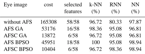
The last experiments, similar to the experiments with iris data, we extended the investigation of AFS and AFSC to more realistic eye image data. Figure 8 and 9 show that BPSO can achieve better results and converge faster than GA. The best feature subset of 10 runs obtained by AFS using GA is five features from Gabor jets (2, 5, 8, 9, 11, 12), four fea-tures from ELAC (14, 17, 20, 21), and six feafea-tures from LOC (48, 51, 53, 54, 56, 57). By applying BPSO, the selected features are three features from Gabor (10, 11, 12), three fea-tures from ELAC (17, 21, 23), and 12 feafea-tures from LOC (29, 32, 38, 39, 47, 48, 49, 50, 51, 53, 54, 57). The AFSC em-ploying both BPSO and GA can select low cost and more less number of features, i.e., only 6 of 58 features. The features 17, 21, 22, 35, 38 and 58 were obtained by using GA and the features 21, 27, 29, 43, 46, and 54 were selected by us-ing BPSO, where the selected features are lower cost features than GA. The recognition rate results for three classification models are summarized in Table 2.
6 Conclusions
The design of sensor systems for recognition tasks can be optimized by eliminating several processing methods and/or sensors that are related to irrelevant features. The goal of this paper was to investigate and show the effectiveness of the automated feature selection with acquisition cost based on aggregation method, in particular employing and comparing two techniques from evolutionary computation, i.e., genetic algorithm and binary particle swarm optimization. The ex-Fig. 7. The average fitness curves of AFSC applying BPSO and GA
for iris train dataset with cost assignment I.
the ELAC, each pixel products with first order neighbors is computed according to masking information. For instance, left and right neighbors will be multiplied with the center pixel for a horizontal mask. From the number of possible masks only 13 significant masks have been chosen here. At each pixel position of the grey value image blocks, all masks will be applied and in a competitive scheme, the strongest response will determine the winning mask. A histogram of all masks keeps track of the frequency of occurrence of mask activation. So the bins of this histogram serve as the fea-tures of the ELAC operator. The LOC operator also work in computation with the first order neighborhood. In contrast to ELAC for investigated mask patterns, no multiplications take place, but pixel differences are computed to determine mono-tonicity. Overall 33 mask patterns are computed at each pixel position. Again, the histogram is computed for the whole re-gion. The cost assignment for the three feature computation operators is determined with regard to the number of multi-plication and addition operations. The assuming multiplica-tion has the cost of 10 addimultiplica-tions. Therefore, the cost of each feature for Gabor filter is 6358, for ELAC 3179 per feature, and 1445 per feature for LOC.
In our experiments, the training datasets are used to find the best feature subset using the AFS optimized by GA and BPSO. Then, the classification models are trained with re-gard to the selected features and tested by using the test
K. Iswandy and A. Koenig: Feature Selection with Acquisition Cost 5
0 20 40 60 80 100 0.972 0.974 0.976 0.978 0.98 0.982 0.984 iteration fitness value BPSO GA
Fig. 6. The average fitness curves of AFS applying BPSO and GA
for iris train dataset.
0 20 40 60 80 100 0.88 0.9 0.92 0.94 0.96 0.98 iteration fitness value BPSO GA
Fig. 7. The average fitness curves of AFSC applying BPSO and GA
for iris train dataset with cost assignment I.
feature for Gabor filter is 6358, for ELAC 3179 per feature, and 1445 per feature for LOC.
In our experiments, the training datasets are used to find the best feature subset using the AFS optimized by GA and BPSO. Then, the classification models are trained with re-gard to the selected features and tested by using the test datasets. Here, we used k-nearest neighbor (kNN), reduced nearest neighbor (RNN), and backpropagation neural net-works (NN) for our classification models. The number of nearest neighbors in kNN is set tok = 9and the Euclidean distance is employed. More extensive experiments and sim-ulations have shown, that for the given data the choice of k and the metric has impact on the results. The reduced-nearest neighbors (RNN) using Euclidean distance, and backpropa-gation neural networks (NN) with one hidden-layer in a x-4-3 network topology for iris data and x-4-2 network topology for eye data. The Levenberg-Marquardt method has been em-ployed for learning.
In the first experiments, the AFS and AFSC optimized by BPSO and GA are investigated for the training enlarged iris dataset with applied 10 different initializations and the results are compared. Figure 6 and 7 show that the average curves of BPSO can converge faster than GA. Both BPSO and GA in optimizing AFS obtained equally the best feature subset. The features 3, 4, 8, 12, and 16 for the enlarged iris data are chosen by AFS. The features 7 and 12 for cost assignment I are found by the AFSC. For cost assignment II the features 2 and 12 are selected. The recognition rate results for three
Table 1. The best run results for iris data. Both BPSO and GA
achieved same results
Iris cost selected k-NN RNN NN
I/II features (%) (%) (%)
without AFS 156/165 16/16 94.67 93.33 93.33
AFS 65/95 5/16 94.67 96.00 94.67
AFSC (I) 7/- 2/16 94.67 97.33 97.33
AFSC (II) -/16 2/16 94.67 93.33 94.67
0 20 40 60 80 100 0.95 0.96 0.97 0.98 0.99 1 iteration fitness value BPSO GA
Fig. 8. The average fitness curves of AFS applying BPSO and GA
for eye train dataset.
classification models are summarized in Table 1.
The last experiments, similar to the experiments with iris data, we extended the investigation of AFS and AFSC to more realistic eye image data. Figure 8 and 9 show that BPSO can achieve better results and converge faster than GA. The best feature subset of 10 runs obtained by AFS using GA is five features from Gabor jets (2, 5, 8, 9, 11, 12), four fea-tures from ELAC (14, 17, 20, 21), and six feafea-tures from LOC (48, 51, 53, 54, 56, 57). By applying BPSO, the selected features are three features from Gabor (10, 11, 12), three fea-tures from ELAC (17, 21, 23), and 12 feafea-tures from LOC (29, 32, 38, 39, 47, 48, 49, 50, 51, 53, 54, 57). The AFSC em-ploying both BPSO and GA can select low cost and more less number of features, i.e., only 6 of 58 features. The features 17, 21, 22, 35, 38 and 58 were obtained by using GA and the features 21, 27, 29, 43, 46, and 54 were selected by us-ing BPSO, where the selected features are lower cost features than GA. The recognition rate results for three classification models are summarized in Table 2.
6 Conclusions
The design of sensor systems for recognition tasks can be optimized by eliminating several processing methods and/or sensors that are related to irrelevant features. The goal of this paper was to investigate and show the effectiveness of the automated feature selection with acquisition cost based on aggregation method, in particular employing and comparing two techniques from evolutionary computation, i.e., genetic algorithm and binary particle swarm optimization. The
ex-Fig. 8. The average fitness curves of AFS applying BPSO and GA for eye train dataset.
6 K. Iswandy and A. Koenig: Feature Selection with Acquisition Cost
0 20 40 60 80 100 0.8 0.85 0.9 0.95 1 fitness value iteration BPSO GA
Fig. 9. The average fitness curves of AFSC applying BPSO and GA
for eye train dataset.
Table 2. The best run results for eye data.
Eye image cost selected k-NN RNN NN
features (%) (%) (%)
without AFS 165308 58/58 96.72 80.33 97.87
AFS GA 53176 16/58 98.36 95.08 96.81
AFSC GA 13872 6/58 96.72 95.08 96.81
AFS BPSO 45951 18/58 100 95.08 98.94
AFSC BPSO 10404 6/58 96.72 98.36 98.94
periments, based on benchmark data (iris data) and more re-alistic eye image data, gave evidence that the achieved results of AFSC employing binary particle swarm are more robust and competitive with regard to speed, classification accuracy and low cost of selected features than GA to effectively op-timize the design of recognition systems. In this paper, our approach only considered to optimize the recognition system according to the cost per feature.
In future work, the extension of the cost and feature group-ing (Pacl´ık et al., 2002) in the selection process and the in-clusion of several additional assessment functions in a multi-objective optimization based on pareto approach (Zitzler and Thiele, 1999) with regard to increasing accuracy and reli-ability will be subject of investigation. In addition to our investigations of the automatic feature selection with acqui-sition cost using GA and BPSO in real applications, the op-timization of multi sensor system in particular to gas sensing (Iswandy et al. , 2005) will also be considered.
References
Agrafiotis, D. K. and Cedeno, W. J.: Feature Selection for Structure - Activitiy Correlation Using Binary Particle Swarms, J. Med. Chem., 45, pp. 1098–1107, 2002
Aha, D. W.: Feature Weighting for Lazy Learning Algorithms, edited by: Liu and Motoda, pp. 13–29, Kluwer Academic Pub-lishers, 1998.
Goldberg, D. E.: Genetic Algorithms in Search, Optimization, and Machine Learning, Addison-Wesley Publishing Company, Inc., 1989.
Jain, A. and Zongker, D.: Feature Selection: Evaluation, appli-cation, and small sample performance, IEEE Trans. on Pattern Analysis and Machine Intelligence, 19(2), pp. 153–158, 1997. Jain, A., Duin, R. and Mao, J.: Statistical Pattern Recognition: a
Re-view, IEEE Trans. on Pattern Analysis and Machine Intelligence, 22(1), pp. 4–37, 2000.
Kennedy, J. and Eberhart, R. C.: Particle Swarm Optimization, in Proc. of IEEE Int. Conf. on Neural Networks (ICNN), 4, pp. 1942–1948, 1995.
Kennedy, J. and Eberhart, R. C.: A Discrete Binary Version of The Particle Swarm Algorithm, Proc. of Conf. on System, Man, and Cybernetics, pp. 4104–4109, 1997.
Koenig, A.: A Novel Supervised Dimensionality Reduction Tech-nique by Feature Weighting for Improved Neural Network Clas-sifier Learning and Generalization, in Proc. of the 6th Int. Conf. on Soft-Computing and Information/Intelligent Systems IIZUKA2000, Iizuka, Fukuoka, Japan, October, pp. 746–753, 2000.
Koenig, A.: Dimensionality Reduction Techniques for Interactive Visualization, Exploratory Data Analysis, and Classification, in: Pattern Recognition in Soft Computing Paradigm, World Scien-tific, FLSI Soft Computing Series (2001), Nikhil R. Pal (Ed.), 2, pp.1–37, 2001.
Koenig, A., Mayr, C., Bormann, T. and Klug, C.: Dedicated Imple-mentation of Embedded Vision Systems Employing Low-Power Massively Parallel Feature Computation, in: Proc. of the 3rd VIVA-Workshop on Low-Power Information Processing, Chem-nitz, Germany, pp. 1–8, 2002.
Koenig, A. and Gratz, A.: Advanced Methods for the Analysis of Semiconductor Manufacturing Process Data, in: Advanced Techniques in Knowledge Discovery and Data Mining, N. R. Pal, L. C. Jain (eds.), pp. 27–74, Springer Verlag, 2005.
Kohavi, R. and John, G. H.: The Wrapper Approach, in: Feature Extraction, Construction and Selection, Liu and Motoda (eds.), pp. 33–50, Kluwer Academic Publishers, 1998.
Iswandy, K., Koenig, A., Fricke, T., Baumbach, M., and Schuetze, A.: Towards Automated Configuration of Multi-Sensor Systems Using Evolutionary Computation - A Method and a Case Study, in printing for J. Computational and Theoretical Nanoscience, December, 2005.
Langley, P.: Elements of Machine Learning, Morgan Kaufmann Publishers, 1996.
Mao, K. Z.: Fast Orthogonal Forward Selection, IEEE Trans. on Neural Networks, 13(5), pp. 1218–1224, 2002.
Pacl´ık, P., Duin, R. P. W., van Kempen, G. M. P., and Kohlus, R.: On Feature Selection with Measurement Cost and Grouped Features, T.Caelli et al. (Eds.): SSPR&SPR 2002, LNCS 2396, pp. 461– 469, Springer-Verlag, 2002.
Siedlecki, W. and Sklansky, J.: On Automatic Feature Selection, Int. J. Pattern Recognition, 2, pp. 197–220, 1988.
Siedlecki, W. and Sklansky, J.: A Note on Genetic Algorithm for Large Scale Feature Selection, Pattern Recognition Letters, 10, pp. 335–347, 1989.
Yang, J. and Honavar, V.: Feature subset selection using a genetic algorithm, in: Feature Extraction, Construction and Selection, Liu and Motoda (eds.), pp. 117–136, Kluwer Academic Publish-ers, 1998.
Zitzler, E. and Thiele, L.: Multiobjective Evolutionary Algorithms: a Comparative Case Study and the Strength Pareto Approach, IEEE Trans. on Evolutionary Computation, 3(4), pp. 257–271, 1999.
Fig. 9. The average fitness curves of AFSC applying BPSO and GA for eye train dataset.
datasets. Here, we used k-nearest neighbor (kNN), reduced nearest neighbor (RNN), and backpropagation neural net-works (NN) for our classification models. The number of nearest neighbors in kNN is set tok=9 and the Euclidean distance is employed. More extensive experiments and sim-ulations have shown, that for the given data the choice of k and the metric has impact on the results. The reduced-nearest neighbors (RNN) using Euclidean distance, and backpropa-gation neural networks (NN) with one hidden-layer in a x-4-3 network topology for iris data and x-4-2 network topology for eye data. The Levenberg-Marquardt method has been em-ployed for learning.
In the first experiments, the AFS and AFSC optimized by BPSO and GA are investigated for the training enlarged iris dataset with applied 10 different initializations and the results are compared. Figures 6 and 7 show that the average curves of BPSO can converge faster than GA. Both BPSO and GA in optimizing AFS obtained equally the best feature subset. The features 3, 4, 8, 12, and 16 for the enlarged iris data are chosen by AFS. The features 7 and 12 for cost assignment I are found by the AFSC. For cost assignment II the features 2 and 12 are selected. The recognition rate results for three classification models are summarized in Table 1.
The last experiments, similar to the experiments with iris data, we extended the investigation of AFS and AFSC to more realistic eye image data. Figures 8 and 9 show that