ORIGINAL ARTICLE
A New Flexible Multibody Dynamics
Analysis Methodology of Deployable Structures
with Scissor-Like Elements
Qi’an Peng
*, Sanmin Wang, Changjian Zhi and Bo Li
Abstract
There are vast constraint equations in conventional dynamics analysis of deployable structures, which lead to dif-ferential-algebraic equations (DAEs) solved hard. To reduce the difficulty of solving and the amount of equations, a new flexible multibody dynamics analysis methodology of deployable structures with scissor-like elements (SLEs) is presented. Firstly, a precise model of a flexible bar of SLE is established by the higher order shear deformable beam element based on the absolute nodal coordinate formulation (ANCF), and the master/slave freedom method is used to obtain the dynamics equations of SLEs without constraint equations. Secondly, according to features of deploy-able structures, the specification matrix method (SMM) is proposed to eliminate the constraint equations among SLEs in the frame of ANCF. With this method, the inner and the boundary nodal coordinates of element character-istic matrices can be separated simply and efficiently, especially on condition that there are vast nodal coordinates. So the element characteristic matrices can be added end to end circularly. Thus, the dynamic model of deployable structure reduces dimension and can be assembled without any constraint equation. Next, a new iteration procedure for the generalized-α algorithm is presented to solve the ordinary differential equations (ODEs) of deployable struc-ture. Finally, the proposed methodology is used to analyze the flexible multi-body dynamics of a planar linear array deployable structure based on three scissor-like elements. The simulation results show that flexibility has a significant influence on the deployment motion of the deployable structure. The proposed methodology indeed reduce the difficulty of solving and the amount of equations by eliminating redundant degrees of freedom and the constraint equations in scissor-like elements and among scissor-like elements.
Keywords: Flexible multibody dynamics, Scissor-like elements, Absolute nodal coordinate formulation, Specification matrix method, Ordinary differential equations
© The Author(s) 2019. This article is distributed under the terms of the Creative Commons Attribution 4.0 International License (http://creat iveco mmons .org/licen ses/by/4.0/), which permits unrestricted use, distribution, and reproduction in any medium, provided you give appropriate credit to the original author(s) and the source, provide a link to the Creative Commons license, and indicate if changes were made.
1 Introduction
Due to their good characteristics such as simple struc-ture, high loading capacity and excellent equilibrium stability [1], deployable structures comprised of SLEs are widely used in many fields, such as architecture [2], antivibration [3] and astronautics [4]. So a great many literatures about configuration design [5, 6], kinematic analysis [7–9] and static analysis [10] of deployable struc-tures with SLEs are published in recent years. As they are used in aerospace engineering field, the space industry is
eager for the prediction of the dynamics features of the deployment process of deployable structures with SLEs. Therefore, Sun [11] proposed a simple way based on the screw theory to study the rigid body dynamics of a spa-tial deployable structure with SLEs. Li [12] researched dynamic characteristics of the deployment process of a planar deployable structure constituted by SLEs with joint clearance. In their researches, the deployable struc-tures with SLEs are regarded as rigid bodies, so elastic vibration and deformation are ignored for dynamics. In order to ensure that the dynamics features of the deploy-ment process of deployable structures with SLEs are fore-casted accurately, regarding them as flexible systems is significant and necessary.
Open Access
*Correspondence: [email protected]
Now there are three main methods on simulating the dynamics of flexible systems [13]. The first one is the floating reference frame approach [14, 15], which is most frequently used because the formulation includes coupling effect between rigid body motions in global coordinate system and small deformations in reference coordinate system connected to the body. However, the formulation deficient in dynamic stiffening will lead to an imprecise simulation result. The second one is the large rotation vector approach [16], but it is used finite ele-ment commercial packages and satellite antenna system frequently. The last one used to describe flexible systems is the absolute nodal coordinate formulation [17–21], in which the displacement gradients at the nodes replace the infinitesimal and finite rotations in conventional finite element [22]. Since the locations at the arbitrary point of the finite element in the formulation are defined in the global coordinate system by using the shape func-tion and nodal coordinates, a constant mass matrix is produced and the Coriolis and centrifugal forces also vanish. Besides, the elastic force is derived on the basis of the continuum mechanics theory, so this formula-tion satisfies the dynamic stiffening automatically and is more exact than the first approach [23]. Therefore, many researches about ANCF have been carried out in all aspects to develop this formulation. For example, other practical elements but beam elements are proposed [24,
25], while performance of element is improved [26] and validated by experiments [27]. More recently, dynamics analysis of deployable structures considering flexibility based on ANCF has become hot areas. Tian et al. [28,
29] applied the absolute nodal coordinate formulation into the dynamics analysis of deployment structures, and the deployment simulations of two kinds of deployable structures in the absolute nodal coordinate frame were carried out as examples. Shan et al. [30] investigated the deployment dynamics of the tethered-net based on abso-lute nodal coordinate formulation, also. However, in their model the dynamics equations are differential-algebraic equations, which are solved hard. To reduce the difficulty of solving and the amount of equations, a new flexible multibody dynamics analysis methodology of deployable structures is presented in this paper.
This paper is organized as follows. Utilizing the higher order shear deformable element based on ANCF, a more exact flexible model of a SLE, in which the constraint equa-tions vanish with the master/slave freedom method, is first established. Then a simple way, SMM, is proposed to separate the inner and the boundary nodal coordinates to obtain the rearranged element characteristic matrices effi-ciently. And based on the rearranged matrices the dynam-ics equations of deployable structures that consist of SLEs are assembled without any constraint equation. Therefore,
a new iteration procedure for the generalized-α algorithm is presented to solve the ODEs. It demonstrates that with the algorithm, the fake high-frequency responses are dissi-pated by numerical examples and the exact analysis results are illustrated. Finally, some main conclusions are drawn.
2 Flexible Dynamics Equations of SLE
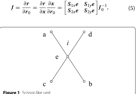
The SLE is basic unit of the deployable structures, which consists of two bars with a middle hinge, as shown in Fig-ure 1. And at tip of each bar, there is a hole, which is used to connect to ground or other SLE. Therefore, a SLE can be decomposed into two same individual links and each link is discretized and modeled in term of ANCF.
In order to avoid the locking problem, a higher order element is used [31], so the global position of an arbitrary point in any beam element is interpolated as follows:
where S is the element shape function, e is the element
coordinate vector. According to the higher order beam element, the coordinate vector can be defined as follow-ing vector
where rα(α=1, 2) is the global position of node 1 and 2, x, y are the element coordinates in the element local coordinate system. The velocity at any material point is obtained
Thus, the kinetic energy of the beam element is given by
where ρ denotes the material density, V denotes the
vol-ume of the element.
The deformation gradient can be defined by continuum mechanics theory
(1)
r=Se,
(2)
e=r1 ∂∂xr1 ∂∂yr1 r2 ∂∂xr2 ∂∂yr2 ∂y∂x∂r1
,
(3)
˙ r=Se.˙
(4)
T =
e Te=
e
1 2
V
ρe˙TSTSe˙dV,
(5)
J = ∂r ∂r0
= ∂r ∂x
∂x ∂r0
=
S1xe S1ye S2xe S2ye
J−10 ,
i
a
d
c
b
e
where Six and Siy is the derivative matrix of the ith row of the beam element shape function with respect to x=x yT respectively, J0=∂r0/∂x and r0=Se0,e0 is the element coordinate vector in the initial configura-tion. Hence, the green strain tensor can be written as
where
and I is an identity matrix. In order to determine the
stress simply, the strain tensor is written in a vector form as
where ε1= 12eTSae−1, ε2= 12eTSbe−1
, and ε3= 12eTSce.
In accordance with constitutive relation, the stress vector is expressed as
where D indicates coefficient matrix of material elastic-ity, and in the case of isotropic homogenous material, its expression is
where
E and ν indicate elastic modulus and the Poisson’s ratio of the beam material respectively. So the strain energy of the beam is obtained:
(6)
ε= 1 2
JTJ−I= 1
2
eTSae−1 eTSce eTSce eTSbe−1
,
Sa=
2
i=1
STixSixcos2θ−STixSiysinθcosθ
− STiySixsinθcosθ+STiySiysin2θ,
Sb=
2
i=1
STixSixsin2θ+STixSiysinθcosθ
+ STiySixsinθcosθ+STiySiycos2θ,
Sc=
2
i=1
STixSixsinθcosθ +STixSiycos2θ
− STiySixsin2θ −STiySiysinθcosθ,
(7)
ε=ε1 ε2 ε3T,
(8)
σ =Dε,
(9)
D=
+2µ 0
+2µ 0
0 0 2µ
,
= Eν
[(1+ν)(1−2ν)],
µ= E
2(1+ν),
Therefore, the dynamics equations of a link of the SLE will be
where me , ke , fe and qe are mass matrix, stiffness matrix, force matrix and generalized coordinate vector of the link, respectively. Thereout, the dynamics equations of the SLE are assembled from two individual links in con-ventional way.
where mg , kg , fg and qg are mass matrix, stiffness matrix,
force matrix and generalized coordinate vector of the SLE, respectively. is the constraint equation, q is the
derivative matrix of with respect to qg.
Because of the middle hinge of the SLE, there is a con-straint equation in the Eq. (12) assembled in a conventional way, and it, the differential-algebraic equations, will lead to solving difficultly. So the master/slave freedom method is introduced to remove the constraint equation.
where q0 indicates the coordinate vector separated from the master/slave freedom vector, qm indicates the master freedom vector and qs indicates the slave freedom vector. So the ordinary differential equations of the SLE is given by
where
3 Flexible Dynamics Equations of Deployable Structures with SLEs
The dynamics equations of the deployable structures arrayed by a large number of SLEs include quite a few constraint equations under assembling by the conven-tional way as a result of the hinges used to connect reciprocally at the tip of bars of SLEs. As mentioned above, the differential-algebraic equations of dynamics
(10)
U =
e Ue=
e 1 2 V
εTσdV.
(11)
meq¨e+keqe=fe,
(12)
mgq¨g+kgqg+q=fg,
�
qg,t�=0,
(13)
qg = q0 qm qs = I 0 0 I 0 I � q0 qm � =Cqp,
(14)
mpq¨p+kpqp=fp,
mp=CTmC,
kp= CTkC,
are tough to solve. In order to reduce dimensionality, i.e., remove the constraint equations, in this paper, a simple and efficient method, SMM, is proposed, which is used to separate the inner and the boundary nodal coordinates. The SMM is stated in detail as follows.
3.1 Specification Matrix Method
If the coordinate vector of some finite element is
and the uniform form having been separated the inner and the boundary nodal coordinates is
Now there is a relationship between primary coordinate vector and the current coordinate vector
where B is a rearranged matrix. In order to obtain the
matrix, B is assumed as a one matrix firstly
Then constraint condition is set by
where i,j=1, 2, 3,. . .,n.
In the end, a calculation procedure is given to improve the efficiency, as shown in Figure 2.
(15)
qo =q1 q2 · · · qi · · · qn,
(16)
q′=
q′
1 q2′ · · ·
Former boundary
· · · q′
i · · ·
Inner nodal coordinates · · · q′
n−1 q′n
Later boundary
.
(17)
qo =Bq′,
(18) B=
b11 b12 · · · b1i · · · b1n
b21 b22 · · · b2i · · · b2n . . . . . . . . . . . .
bi1 bi2 · · · bii · · · bin . . . . . . . . . . . .
bn1 bn2 · · · bni · · · bnn =
1 1 · · · 1 · · · 1 1 1 · · · 1 · · · 1
. . . . . . . . . . . . 1 1 · · · 1 · · · 1
. . . . . . . . . . . . 1 1 · · · 1 · · · 1
. (19)
bij·qj′=qi⇒bij=1,
bij·q′j�=qi ⇒bij=0, n
�
i=1
bij =1,
n �
j=1
bij =1,
3.2 Flexible Dynamics Equations of Deployable Structures with SMM
The uniform form of the generalized coordinate vector of the SLE is
Based on SMM, the rearranged matrix B is obtained, and the dynamics equations of the SLE in this case are rewrit-ten as
where
The dynamics equations of the deployable structures with SLEs are expressed as [32]
where
(20)
qb=B−1qp.
(21)
mbq¨b+kbqb=fb,
mb=BTmpB,
kb=BTkpB,
fb=BTfp.
(22)
Mq¨+Kq=Q,
M=
N
i=1
TTi mibTi,
K =
N
i=1
TTi kibTi,
Q=
N
i=1 TTi fib,
q denotes the generalized coordinate vector of the deployable structures with the SLEs, N is the number of SLEs and T denotes the element Boolean matrix.
4 Solution to Flexible Dynamics Model
Based on the formulation, the dynamics equations of the deployable structures with SLEs have been changed into ordinary differential equations from the differential-alge-braic equations. Hence, the dynamics equations are solved more easily. However, numerical results are unsatisfactory by using classical numerical approach to solve the dynam-ics equations, because of the high-frequency response in the results. So the generalized-α method is used to solve the equations, meanwhile dissipate the fake high-fre-quency response which occurs since the finite element dis-cretization, while well preserve the realistic motions. The basic form of the generalized-α algorithm is given by
Note that a is an auxiliary variable, it is defined by the recurrence relation
where n denotes the nth iteration, β , γ , αm , αf are the
algo-rithm parameters. In order to make the method uncon-ditionally stable, second-order accurate, and an optimal combination of the high-frequency dissipation and the realis-tic motion preservation, the parameters in the generalized-α
algorithm should be met the relations as follows [33]
where α∈0 1 . As α increases from 0 to 1, the
perfor-mance dissipating the high-frequency response reduces. α=0 is the asymptotic annihilation case, while α=1 leads to no dissipation case. The generalized-α algo-rithm is used to solve the structural dynamics initially, and Arnold proposed a computational scheme extend it to dynamics with constraint equations [34]. In this paper, some improvements for the scheme are given to fit the
(23)
qn+1=qn+hq˙n+h2
1 2 −β
an+h2βan+1,
˙
qn+1= ˙qn+h(1−γ )an+hγan+1.
(24)
(1−αm)an+1+αman=1−αf
¨
qn+1+αfq¨n,
a0=q¨0,
(25)
γ =1
2−αm+αf,
β=1
4
1−αm+αf2,
αm=
2α−1
α+1 ,
αf =
α
α+1,
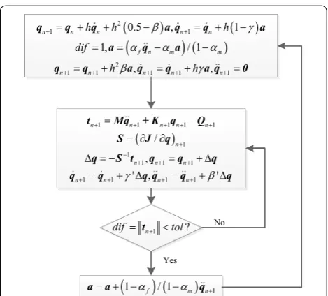
ordinary differential equations, and the improved scheme is illustrated as Figure 3.
In Figure 3, β′= 1−αm
h2β1−α f and γ
′= γ
hβ . Besides, tol is
the integration error tolerance, S is the Jacobian matrix of
J and J is given by
5 Numerical Example
As a numerical example, the dynamics analysis of a deployable structure assembled by three individual SLEs is carried out. As shown in Figure 4, the global coordi-nates system’s origin locates point b1 , and the driving force equaled to 50 N applies at point a1 . In order to
avoid the locking problem, the Poisson’s ratio is set to zero. The other parameters of deployable structure are shown in Table 1.
(26)
J =Mq¨+Kq−Q.
Figure 3 The numerical iteration procedure of the generalized-α algorithm
F
X
O
1
2
Y
3
θ
a
1a
2a
3a
4b
1b
2b
3b
4c
1c
2c
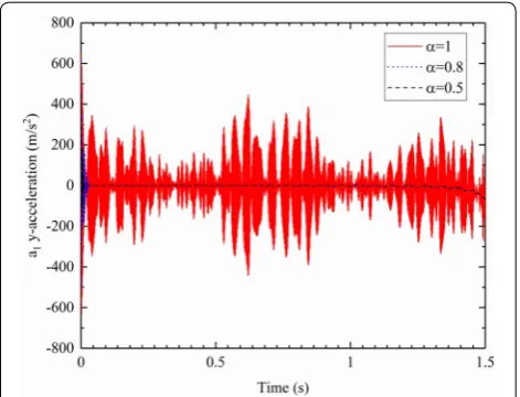
3From Figure 5, the high-frequency response is dissipated by choosing an appropriate α with the generalized-α method. On the other hand, Figure 6
shows that the realistic motion of point a1 is well pre-served despite the fact that the high-frequency energy is dissipated.
Figure 7 shows the difference of the dynamics of the deployable structure with three SLEs between flexible and rigid system. It is clear that under constant driving force the deployment process of the deployable structure is variable accelerated motion in both cases. In addition, their displacement, velocity and acceleration change very quickly within the last 0.3 s. However, from Figure 7c–f, compared with rigid body, apparent vibration appears on velocity and acceleration due to flexibility of the deploy-able structure, and the maximum amplitudes are 0.3889 m/s and 18.60 m/s2, respectively. It should be noted that the vibration also exist in displacement, but it is too small to observe. Another a key difference seen from Figure 7a and b is different displacement between flexible and rigid deployable structure, because the flexible body is sub-jected to the coupling of tensile deformation, shear defor-mation and bending defordefor-mation. And the maximum difference value in x-direction displacement is 0.01498 m, while the maximum difference value in y-direction dis-placement is 0.02503 m.
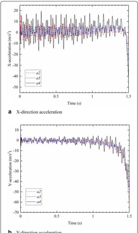
Figures 8, 9, 10 show the displacement, velocity and acceleration of point a2 , point a3and point a4 in the case of flexibility. Figure 8b shows that y-displacement is obvi-ously non-synchronous after 1.20 s because of different degrees of deformation caused by velocity and accel-eration increasing fast in the late period of deployment. And the maximum differences equal 0.01863 m between point a2 and point a3 and 0.02203 m between point a3and point a4 , respectively. Both of them happen at 1.5 s. Also, the y-velocity, whose differences vary from 0 to 0.7749 m/s, and y-acceleration, whose differences vary from 0 to 27.20 m/s2, are not synchronous anymore from Fig-ure 9b and from Figure 10b due to flexibility. Combined with Figure 8 to Figure 10, it is easily inferred that as the number of the SLE making up of the deployable struc-ture increases, the vibration of displacement, velocity,
acceleration and deformation of the flexible system are more obvious.
6 Conclusions
This paper presents a new dynamics analysis methodol-ogy for deployable structures with SLEs on the basis of the ANCF, and the availability of the proposed methodol-ogy is verified by a numerical example. We can have the conclusions as follows.
(1) In the analysis methodology, the master/slave free-dom method is introduced to eliminate the con-straint equations in SLE. The SMM is proposed to eliminate the constraint equations among SLEs in the frame of ANCF, which can separate the inner Table 1 Material properties and geometry sizes
of the deployable structure
Characteristic parameter Value
link length L (m) 1
cross-sectional area A (m2) 0.02 × 0.02
material density ρ (kg/m3) 2750
elasticity modulus E (N/m2) 7 × 10¹⁰
Poisson’s ratio ν 0
Figure 5 Y-direction acceleration of point a1
and the boundary nodal coordinates simply and efficiently.
(2) By utilizing the methodology, the element char-acteristic matrices can be added end to end circu-larly and the redundant degrees of freedom of the dynamics equations of the deployable structures can be eliminated, so then the equations can turn into ODEs from DAEs. Thus, the expressions of the dynamics equations become simpler and the alter-native solutions are more, it also means that the difficulty to solve reduces. Besides, the methodol-ogy can be extended to flexible analysis of the other types of deployable structures.
(3) The generalized-α method is introduced and an improved computational scheme for the method
is used to solve the ordinary differential dynamics equations. It is shown that the improved compu-tational scheme is valid and the realistic motion is well preserved despite the high-frequency energy is dissipated by using the method.
m + 0.02203 m) = 0.04066 m. Therefore, it is con-firmed that flexibility has a significant influence on the dynamic performance, such as smoothness and synchronism of deployment process of deployable structures with SLEs.
Abbreviations
DAEs: differential-algebraic equations; SLEs: scissor-like elements; ANCF: abso-lute nodal coordinate formulation; SMM: specification matrix method; ODEs: ordinary differential equations.
Authors’ contributions
QP proposed the analysis methodology and wrote the manuscript; SW refined the methodology; CZ proofreaded the manuscript; BL wrote the program. All authors read and approved the final manuscript.
Authors’ Information
Qi’an Peng, born in 1993, is currently a PhD candidate at School of Mechanical Engineering, Northwestern Polytechnical University, China. His main research internets include space deployable structure and multi-bodies systems dynamics.
Sanmin Wang, born in 1961, is currently a professor at School of Mechanical Engineering, Northwestern Polytechnical University, China. He received his PhD degree from Northwestern Polytechnical University, China, in 2004.
Changjian Zhi, born in 1984, is currently a PhD candidate at School of Mechanical Engineering, Northwestern Polytechnical University, China.
Bo Li, born in 1986, is currently a PhD candidate at School of Mechanical Engineering, Northwestern Polytechnical University, China.
Competing Interests
The authors declare no competing financial interests.
Funding
Supported by National Natural Science Foundation of China (Grant No. 51175422).
Received: 28 May 2018 Revised: 20 April 2019 Accepted: 4 September 2019
References
[1] W Zhang, J Zhao. Analysis on nonlinear stiffness and vibration isolation performance of scissor-like structure with full types. Nonlinear Dynamics, 2016, 86(1): 1-20.
[2] H Tagawa, N Sugiura, S Kodama. Structural analysis of deployable structure with scissor-like-element in architectural design class. IABSE Conference, Nara, Japan, May 13-15, 2015: 1-8.
[3] X Sun, X Jing. Analysis and design of a nonlinear stiffness and damp-ing system with a scissor-like structure. Mechanical Systems and Signal Processing, 2016, 66: 723-742.
[4] M Takatsuka. General dynamic modeling of a scissor structure for its deployment control in space. International Journal of Space Structures, 2015, 30(3-4): 245-259.
[5] T J Li, H Deng, X Ma, et al. Design and analysis of space deployable anten-nas composed of scissor-like hinges driven by springs. Aiaa/asme/asce/ ahs/asc Structures, Structural Dynamics, and Materials Conference, Boston, Massachusetts, April 8-11, 2013: 1-7.
[6] N Hua, Z Xie, L Luo, et al. Design and analysis in multiple-scissor-linkage applied to the robotics arm. 3rd International Conference on Mechatronics, Robotics and Automation, Bali, Indonesia, October 11-12, 2015: 482-485. [7] J Zhao, Z Feng, F Chu, et al. Advanced theory of constraint and motion
analysis for robot mechanisms. 1st ed. Orlando: Academic Press, Inc., 2013. [8] J Cai, X Deng, J Feng, et al. Mobility analysis of generalized angulated
scissor-like elements with the reciprocal screw theory. Mechanism & Machine Theory, 2014, 82(24): 256-265.
[9] Y Sun, S Wang, J Li, et al. Mobility analysis of the deployable structure of sle based on screw theory. Chinese Journal of Mechanical Engineering, 2013, 26(4): 793-800.
[10] B Li, S M Wang, C J Zhi, et al. Analytical and numerical study of the buckling of planar linear array deployable structures based on scissor-like element under its own weight. Mechanical Systems & Signal Processing, 2016, 83: 474-488.
[11] Y Sun, S Wang, J K Mills, et al. Kinematics and dynamics of deployable structures with scissor-like-elements based on screw theory. Chinese Journal of Mechanical Engineering, 2014, 27(4): 655-662.
[12] B Li, S M Wang, R Yuan, et al. Dynamic characteristics of planar linear array deployable structure based on scissor-like element with joint clearance using a new mixed contact force model. ARCHIVE Proceedings of the Insti-tution of Mechanical Engineers, Part C: Journal of Mechanical Engineering Science 1989-1996 (vols 203-210), 2015, 230(18): 3161-3174.
[13] D Garcíd, A-Vallejo, J Valverde, et al. An internal damping model for the absolute nodal coordinate formulation. Nonlinear Dynamics, 2005, 42(4): 347-369.
[14] P W Likins. Finite element appendage equations for hybrid coordinate dynamic analysis. International Journal of Solids & Structures, 1972, 8(5): 709-731.
[15] J G D Jalón, E Bayo. Kinematic and dynamic simulation of multibody sys-tems. 1st ed. New York: Springer, 1994.
[16] J C Simo, L Vuquoc. On the dynamics of flexible beams under large overall motions—the plane case: Part I and part II. Journal of Applied Mechanics, 1986, 53(4): 849-863.
[17] A Shabana. Dynamics of multibody systems. 3rd ed. Cambridge: Cam-bridge University Press, 2005.
[18] M Berzeri, A A Shabana. Development of simple models for the elastic forces in the absolute nodal co-ordinate formulation. Journal of Sound & Vibration, 2000, 235(4): 539-565.
[19] M A Omar, A A Shabana. A two-dimensional shear deformable beam for large rotation and deformation problems. Journal of Sound & Vibration, 2001, 243(3): 565-576.
[20] R Y Yakoub, A A Shabana. Three dimensional absolute nodal coordinate formulation for beam elements: Implementation and applications. Jour-nal of Mechanical Design, 2001, 123(4): 614-621.
[21] A A Shabana, R Y Yakoub. Three dimensional absolute nodal coordinate formulation for beam elements: Theory. Journal of Mechanical Design, 2001, 123(4): 606-613.
[22] A A Shabana. Definition of the slopes and the finite element absolute nodal coordinate formulation. Multibody System Dynamics, 1997, 1(3): 339-348.
[23] M Berzeri, A A Shabana. Study of the centrifugal stiffening effect using the finite element absolute nodal coordinate formulation. Multibody System Dynamics, 2002, 7(4): 357-387.
[24] M Langerholc, J Slavic, M Boltežar. A thick anisotropic plate element in the framework of an absolute nodal coordinate formulation. Nonlinear Dynamics, 2013, 73: 183-198.
[25] A Olshevskiy, O Dmitrochenko, H-I Yang, et al. Absolute nodal coordinate formulation of tetrahedral solid element. Nonlinear Dynamics, 2017, 88(4): 2457-2471.
[26] H Yu, C Zhao, B Zheng, et al. A new higher-order locking-free beam ele-ment based on the absolute nodal coordinate formulation. Proceedings of the Institution of Mechanical Engineers, Part C: Journal of Mechanical Engineering Science, 2018, 232(19): 3410-3423.
[27] G Orzechowski, J Frączek, T Barczak. Physical experiment and computer simulation of the speed-up manoeuvre using the absolute nodal coor-dinate formulation. Proceedings of the Institution of Mechanical Engineers, Part K: Journal of Multi-body Dynamics, 2018, 232(4): 473-480.
[28] P Li, C Liu, Q Tian, et al. Dynamics of a deployable mesh reflector of satel-lite antenna: Parallel computation and deployment simulation. Journal of Computational and Nonlinear Dynamics, 2016, 11(6): 0610051-06100516. [29] Q Tian, J Zhao, C Liu, et al. Dynamics of space deployable structures. ASME
2015 International Design Engineering Technical Conferences and Computers and Information in Engineering Conference, Boston, USA, 2–5 August, 2015: 1-8.
[30] M Shan, J Guo, E Gill. Deployment dynamics of tethered-net for space debris removal. Acta Astronautica, 2017, 132: 293-302.
[31] J Gerstmayr, A A Shabana. Analysis of thin beams and cables using the absolute nodal co-ordinate formulation. Nonlinear Dynamics, 2006, 45(1-2): 109-130.
[32] J Liu, J Hong. Nonlinear formulation for flexible multibody system with large deformation. Acta Mechanica Sinica, 2007, 23(1): 111-119. [33] J Chung, G M Hulbert. A time integration algorithm for structural
dynam-ics with improved numerical dissipation: The generalized-α method. Journal of Applied Mechanics, 1993, 60(2): 371-375.