www.adv-radio-sci.net/11/113/2013/ doi:10.5194/ars-11-113-2013
© Author(s) 2013. CC Attribution 3.0 License.
Advances in
Radio Science
Simulating circuits with impasse points
T. Thiessen and W. Mathis
Institute of Theoretical Electrical Engineering, Leibniz University of Hannover, Germany Correspondence to: T. Thiessen ([email protected])
Abstract. In this paper circuits with impasse points, i.e. with jumps in their configuration space will be analyzed. These non-regularized circuits exhibit a fold in their configuration space, which can lead to difficulties during the simulation with standard circuit simulators like SPICE. The former de-veloped geometric approach to simulate these circuits with-out regularization will be extended by a detailed discussion of which coordinate system has to be chosen. Furthermore, two new approaches for a numerically efficient calculation of the hit points will be shown.
1 Introduction
There is a class of electronic circuits whose configuration space manifoldSis folded within the embedding spaceEof currents and voltages. This fold can be related to so-called impasse points and leads under certain conditions to jumps from one stable part of S to another. A classical transient solution of such non-regularized circuits exhibiting impasse points is not possible (see e.g. Chua (1980), Reissig (1996), Chua and Deng (1989a)). However, a common method to overcome these simulation problems is to regularize the cir-cuit by adding suitable located parasitic inductors L’s or ca-pacitors C’s considering Tikhonov’s Theorem (for further lit-erature see Reissig (1996)). In previous works, a geometric concept was developed to simulate those circuits without reg-ularization (see e.g. Thiessen and Mathis (2011a), Thiessen et al. (2013)). There, several electronic circuits exhibiting these behavior were studied and different approaches to cal-culateS, jump and hit points were analyzed (e.g. Thiessen et al. (2012b), Thiessen et al. (2012a), Thiessen et al. (2011), Thiessen and Mathis (2011b), Thiessen and Mathis (2011a)). In this work improvements in the topic of hit point calcu-lation will be shown. Especially the difficulty of multiple hit points will be studied in detail. Furthermore, a detailed description of the geometric system analysis will be given. There, the question of which coordinate system, i.e. system
of equations, is best placed to deal with those non generic circuits will be answered.
2 Geometric system analysis
Common circuit simulators (e.g. SPICE) are based on MNA, which leads in the description of electronic circuits to a quasilinear differential-algebraic system of equations (DAE) (cf. Riaza (2008)):
AcC(ATce)ATce˙= −Arγr(ATre)−. . .
. . .−Alil−Auiu−Ajis(t ) (1a)
L(il)˙il=ATl e (1b)
0=vs(t )−ATue (1c)
This system of equations can also be formulated as
B(c)˙c=h(c(t )) . (2)
In the sense of Reich Reich (1990) eq. (2) is a triple (Rk,B,h), where B:Rk→Rk×k is a linear operator and h: Rk→Rka diffeomorphism. Reich had proven that the DAE (2) is regular, if there is a differentiable manifold S⊂Rk
and a vector field v:S→T S, such that a differential map-ping w:I→S (I⊂R) is a solution of the vector field for allt∈I, if and only if the mapping c:j◦w:I→Rkis a so-lution of the DAE, where j:S→Rk is the natural injection Reich (1990).
This work focuses on the investigation of non-regular DAEs where impasse points exists. These impasse points will be called “jump points”, because the transients will be con-tinued by jumps inEfrom one point onSto another.
The systems of equations of the considered nonlinear dy-namical circuits can be characterized by a semi explicit DAE:
˙
x=g(x,y, t ) (3a)
xn ym
zη
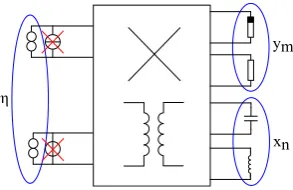
Fig. 1. Network for determiningS
The vector x∈Rn corresponds to the capacitor voltages and inductor currents and the vector y∈Rm to additional voltages and currents in an electronic circuit.
Taken into account thatS can exhibit a fold e.g. respec-tively an input voltage vs(t )and not respectivelyt, the input sources have to be treated differently. For describing the be-havior of the circuit for any input values, the independent and time dependent input sources will be replaced by nora-tors and treated as further vector z fo unknowns (cf. Fig. 1). Therefore, an additional vector z∈Rη has to be consid-ered in the describing system of equations. The resulting autonomous, semi explicit system of equations then is de-scribed by:
˙
x=g(x,y,z) g:Rk→Rn (4a)
0=f(x,y,z) f:Rk→Rm (4b)
These system of Eq. (4) forms the basis of the further inves-tigations. The distinction in x, y and z is essential for calcu-latingS and the jump and hit points.Scan be defined as a subspace ofE=Rk(wherek=n+m+η) and is represented by the solution set of the independent algebraic Eq. (4b). The calculation of the jump and hit points will be shown in Sec-tion 3 and 4.
Remark: As can be seen, the system of equations (1) do not distinct between x, y and z. One method to modify the system of equations (1) to (4) is shown in Thiessen et al. (2012a) and Thiessen et al. (2013). Another method for de-riving a system of equations of type (4) is by applying the Augmented Nodal Analysis (ANA) shown in Riaza (2008). The resulting system of equations derived by the Augmented Nodal Analysis (ANA) is
C(vc)v˙c=ic (5a)
L(il)˙il=ATl e (5b)
0=Arγr(ATre)+Alil+Acic+Auiu+Ajis(t ) (5c) 0=vc(t )−ATce (5d)
0=vs(t )−ATue (5e)
Here, the vectors vc and il are counted among the vector x. The vector y is composed of ic, iuand e and the input vectors isand vs are counted among the vector z.
Ps Pj
S
Ph
JS
y
z x
transient solution jump-set Γ
x x
S
Γ Ps
Pj
(a) (b)
Fig. 2. Calculation principle of (a)Pj and (b)Ph
3 Jump points
It was shown by Chua and Deng (1989b), that almost all sin-gular points of an autonomous semi explicit DAE are in fact impasse points, i.e. jump points. However, e.g. in Chua and Deng (1989a), Chua and Deng (1989b) and Andronov et al. (1966), the fact thatScould contain a fold respectivelyzwas neglected. Taken this into account and knowing that singular points are points, where the local solvability toyis not guar-anteed (e.g. Thiessen et al. (2011), Chua and Deng (1989a)), the necessary jump condition can be specified by (cf. Chua and Deng (1989a), Andronov et al. (1966)):
det ∂yf(x,y,z)
=0 where f(x,y,z)=0 (6)
A point that is specified by eq. (6) and whose neighborhood includes each a Lyapunov-stable and -unstable point, is de-fined as proper jump pointPj. This sufficient jump condi-tion can be verified by calculating the eigenvaluesλi of the characteristic equation det ∂yf(x,y,z)−λ·E=0, where E
is the identity matrix (cf. theory of discontinuous oscillators e.g. Andronov et al. (1966), Mishchenko and Rozov (1980)). The set of all points fulfilling these two conditions is called jump-set0, which represents a l−1-dimensional subset of
S. Of course, the calculation of the zero set of all points ful-filling them+1 algebraic equations specified by Eq. (6) is difficult. However, not all zeros of Eq. (6) are of interest, but only in the actual chosen jump point during a simula-tion. Hence, the dynamics onSwill be traced till reaching a stopping pointPs. This stopping point is defined as a point, where the step size of the numerical solver reaches a lower boundary (which is related to the machine constant of the simulating computer). In the next step, the ”nearest” point on 0will be calculated by choosing a suitable norm and defined as the actual jump pointPj(cf. Fig. 2 (a)).
4 Hit points
use a variable order solver based on the numerical differenti-ation formulas (NDFs) Shampine and Reichelt (1997).
Considering that the voltage across a capacitance and the current through an inductance is preserved, both have iner-tia through a jump process and do not change (i.e.xj=xh). Assuming that a jump happens instantaneous, i.e.tj=th, a further restriction is the fixed value of z (i.e. vs(tj)=vs(th), is(tj)=is(th)) during a jump. Consequently, a jump takes place in a tangential space ofRm, which corresponds to the coordinate space of y. In the following, the jump space will be denoted byJ S. This corresponds to the jump postulate of Chua and Alexander (1971).
Because we introducedE, a hit pointPhcan be calculated by the intersection ofJ Sdefined inPj andSexcluding the jump point itself (Ph∈(J SPj∩S)0) (see Fig. 2 (b)).
Thus, the problem of the hit point calculation can be de-fined as
0=f(xj,y,zj)=:h(y), (7)
with the constraint
yh6=yj . (8)
In Thiessen and Mathis (2011a), Sarangapani et al. and Thiessen et al. (2012a) the hit point calculation was done in two steps: First a point Pj0 outside S was chosen so thatPh0∈(J S0P
j0∩S). In the next step, the actual hit point Ph∈(J SPj∩S)0with the initial conditionPh0 was cal-culated. There, the difficulty was to chose a suitable pointPj0 outsideS, so that the numerical solver is able to findPh0.
Another approach (cf. Thiessen et al. (2011)) to calculate a hit point was to use a bisection method. This provided a set of possible points from which the closest to the corresponding jump point was chosen.
Now, an efficient approach to calculate the hit points of circuits with only one fold inSbased on the penalty function will be shown.
4.1 Penalty function
The basic idea of a penalty function is to convert the zero problem of Eq. (7) with a constraint (8) in a zero problem without constraint (cf. Florian Jarre (2003)).
Thus, the optimization problem
h(y)→min wit h y6=yj , (9)
where h:Rm→Rmcan be transformed to
p(y,r):= [h(y)+r·l(y)] →min . (10) The penalty function p(y,r)consists of the weighted sum of the objective function h(y)and the penalty functionl(y). The penalty function itself can be weighted by the vector r=
(r1, r2, . . . , rm)T which is chosen to be r =r·(1,1, . . . ,1)T in this work.
Here, an easy penalty function for the constraint of eq. (8) was chosen:
l(y)= 1
ky−yjk2 (11)
It follows thatl(y)→0 for y6=yjandl(y)→ ∞for y≈ yj.
To achieve a more robust solution, suitable initial condi-tions yh,0 outsideS has to be chosen. It became apparent,
that the addition of the inverse of the last step 1y to yj, yields a more robust numerical solution than by choosing e.g. yh,0=0. This can be explained by the switching process
of the considered circuits.
FromPhthe dynamics can be traced, till reaching0again.
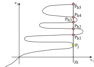
5 Multiple hit points
Another problem appears if the configuration spaceS of the electronic circuit is multiple folded, so that there are multiple possible hit points (cf. Fig. 3).
v2
v1 JS
Pj Ph1 Ph2 Ph4 Ph5
Ph3
Fig. 3. Multiple hit points
In these cases, the penalty function approach is not suit-able and a new approach based on the homotopy method is needed.
5.1 Homotopy method
The homotopy method is used to solve nonlinear algebraic equations of the form (7). The advantage is that the conver-gence region is much larger than the one by applying the penalty approach. Starting from an easy zero problem, the system of equations will be deformed byλtill reaching the original zero problem. This continuous deformation process is achieved by solving H(y, λ)=0. A general homotopy can be given as follows:
H(y, λ)=λh(y)+(1−λ)B(y)=0. (12)
(a) (b) G1(VD1)
I Vsum
G2(VD2)
0 2 4 6 8 10 12
0.2 0.4 0.6 0.8 1 1.2 VDi/V I Di /mA 0 D1 D2
Fig. 4. (a) Analyzed TD circuit; (b) two TD characteristics
The zero curve of the homotopy map H(y, λ)(homotopy path) can be tracked by different techniques. One technique, which is used in this work, is to use an ODE-based algorithm (cf. Watson (1990)). For this, the parametrization is not based onλbut on the arc length s of the homotopy path. There-for, the equation H(y(s), λ(s))=0 has to be differentiated with respect tosand solved forλand y. The main advantage for using the arc length method is because therewith regres-sive homotopy paths can be traced. A disadvantage of such a multiple-step method is, that the error of the approximation of y increases with every step. By using a predictor corrector method, the error accumulation can be counteracted.
In the following the problem of multiple hit points will be displayed by the example of two series connected resonance tunneling diodes (cf. Fig. 4 (a)) Thiessen et al. (2012b). The chosenV-I characteristics of the tunnel diodes is shown in Fig. 4 (b). A good approximation of theseV-Icharacteristics can be achieved by using the following equation (cf. Chang et al. (1993)):
Gj(VDj)=e·
c1·VDj·
h
t an−1(c2·VDj+c3)
−t an−1(c2·VDj+c4) i
+c5·VDjm +c6·VDjl
, (13)
whereci are constants related to the peak and valley currents and voltages, eis a scaling factor and mand l are integer fitting factors.
By using a norator, as explained in Section 2, the con-figuration space S of the series connection can be deter-mined by solving the system of equationsI=G1(VD1), I=
G2(VD2), Vsum=VD1+VD2(cf. Fig. 5).
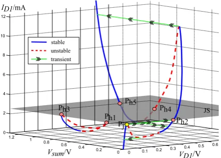
It is noteworthy that the configuration space of the series connection consists of two separated manifolds: one main part proceeding through the origin and a second separated single loop which can only be reached by choosing suitable initial conditions (cf. Thiessen et al. (2012b)). If the current I is increased from zero, the first jump point of the non-regularized circuit of Fig. 4 (a) will be reached at the point Pj. From there, there are five possible hit points as shown in Fig. 5).
For the sake of completeness, the transients of the cor-responding regularized circuit are also shown in Fig. 5) by the green lines with arrows. The regularized circuit can be achieved by adding small capacitances parallel to the diodes (cf. Thiessen et al. (2012b)).
JS
0 0.1 0.2 0.3 0.4 0.5 0.6 0 0.2 0.4 0.6 0.8 1 1.2 0 2 4 6 8 10 12 VD1/V Vsum/V ID1/mA stable unstable transient Pj Ph1 Ph3 Ph2 Ph4 Ph5
Fig. 5.Sof the series connection ofD1 andD2
1 VD1/V VD2/V λ 0.9 0.8 0.7 0.6 0.5 0.4 0.3 0.2 0.1 0
0.998 0.999 1 1.001 1.002 1.003 1.004 1.005 1.006 1.007 1.008 0 0.5 1 1.5 2 Pj Ph2 Ph4 Ph5
Fig. 6. Homotopy path
To calculate the hit points, the FPN homotopy shown in Rahimian et al. (2011) is used. The FPN homotopy con-sists of a combination of the fixed-point (FP) and Newton (N) function approach and can be formulated in two steps: (1) The function h(y)to be solved is multiplied by the fixed-point function giving
hfp(y)=h(y)(y−y0) . (14)
(2) The function B(y) is formed by a combination of the fixed-point and Newton function (cf. Rahimian et al. (2011)) yielding
B(y)=(y−y0)+(hfp(y)−hfp(y0))=0. (15)
Inserting Eq. (14) and eq.(15) in Eq. (12) gives H(y, λ)=λhfp(y)+
(1−λ)· (y−y0)+(hfp(y)−hfp(y0))=0. (16)
After some rearrangements, eq.(16) simplifies to
H(y, λ)=(1+h(y)−λ)·(y−y0) . (17)
in Fig. 6. The jump pointPj was chosen as starting point y0, which is also a solution of h(y). To calculate further
ze-ros except Pj, the homotopy path was progressed beyond λstart=1. Therefore, a bifurcation point (BP) was inserted
atPj(cf. Dhooge et al. (2006)).
The numerical calculation of the homotopy path was done by a numerical continuation method, which includes a pre-dictor corrector method. Therefore, the MATLAB toolbox CL MATCONT was used Dhooge et al. (2006).
As can be seen from Fig. 5 and Fig. 6 not all hit points can be calculated with this method. The hit points on the sep-arated single loop cannot be calculated, but all hit points on the main part ofS. This results due to the fact, thatSconsists of two separated manifolds.
The hit points on the separated single loop are in fact insta-ble points and could be calculated by choosing suitainsta-ble initial conditions. But, for tracking the transients, only the stable hit points are of interest, which arePh2andPh4. Now the
ques-tion is, which of these both points is the right hit point ? In the work of Chua and Alexander (1971) there is an iner-tia postulate which says: trajectories on a stable branch will continue on a stable part till reaching a jump point and than jump to the ”nearest” stable part ofS. But a complete proof of this postulate is still pending. One possibility to verify this postulate is to analyze the catchment area of the dynamic of the corresponding regularized circuit, but this will be the fo-cus on further studies.
6 Conclusions
In this work, a detailed description of the geometric system analysis was given. Thereby it was explained why the system of equations yielding from the ANA is the most suitable for applying the geometric approach. Furthermore, the penalty and the homotopy approach for a numerically efficient cal-culation of the hit points were shown. The penalty function method turned out to be suitable for circuits with only one fold inS, but not for several folded configuration spaces. By using a homotopy method with a proper homotopy function, all hit points can be calculated assumingS consists only of one manifold. In this work a non generic case, whereS con-sists of two separated manifolds was shown. In those cases, not all hit points can be calculated without further arrange-ments. Furthermore, the question of choosing the right hit points appeared, but shall be studied in further investigations.
Acknowledgements. The authors would like to thank the German
Research Foundation (DFG) for the financial support and Serdar Ediz for his valuable contributions to the topic of hit point calcula-tion.
References
Andronov, A., Vitt, A., and Kha˘ıkin, S.: Theory of Oscilators, In-ternational Series of Monographs in Physics, Vol. 4., Pergamon Press Ltd., 1966.
Chang, C., Asbeck, P., Wang, K.-C., and Brown, E.: Analysis of Heterojunction Bipolar Transistor/Resonant Tunneling Diode Logic for Low-Power and High-Speed Digital Applications, IEEE T. Electr. Dev., 40, 685–691, 1993.
Chua, L.: Dynamic nonlinear networks: State-of-the-art, IEEE T. Circuits Syst., 27, 1059–1087, 1980.
Chua, L. and Alexander, G.: The Effects of Parasitic Reactances on Nonlinear Networks, IEEE T. Circuits Syst., 18, 520–532, 1971. Chua, L. O. and Deng, A.-C.: Impasse Points. Part 1: Numerical As-pects, International Journal of Circuit Theory and Applications, 17, 213–235, 1989a.
Chua, L. O. and Deng, A.-C.: Impasse Points, Part 2: Analytical Aspects, Int. J. Circ. Theor. App., 17, 271–282, 1989b.
Dhooge, A., Govaerts, W., Kuznetsov, Y. A., Mestrom, W., Riet, A. M., and Sautois, B.: MATCONT and CL MATCONT: Con-tinuation toolboxes in matlab, 2006.
Florian Jarre, J. S.: Optimierung, Springer-Verlag, 2003.
Mishchenko, E. F. and Rozov, N. K.: Differential Equations with Small Parameters and Relaxation Oscillators, Plenum Press, 1980.
Rahimian, S. K., Jalali, F., Seaderc, J., and White, R.: A new homo-topy for seeking all real roots of a nonlinear equation, Computers and Chemical Engineering, 35, 403–411, 2011.
Reich, S.: On a Geometrical Interpretation of Differential-Algebraic Equations, Circ. Syst. Sign. Pr., 9, 367–382, 1990.
Reissig, G.: Differential-Algebraic Equations and Impasse Points, IEEE T. Circuits Syst., 43, 122–133, 1996.
Riaza, R.: Differential-Algebraic Systems: Analytical Aspects and Circuit Applications, World Scientific, 2008.
Sarangapani, P., Thiessen, T., and Mathis, W.: Differential Alge-braic Equations of MOS Circuits and Jump Behavior (accepted), Advances in Radio Science.
Shampine, L. F. and Reichelt, M. W.: The MATLAB ODE Suite, SIAM Journal on Scientific Computing, 18, 1–22, 1997. Thiessen, T. and Mathis, W.: Geometric Dynamics of Nonlinear
Cir-cuits and Jump Effects, International Journal of Computations & Mathematics in Electrical & Electronic Engineering (Compel 2011), 30, 1307–1318, 2011a.
Thiessen, T. and Mathis, W.: Geometrical Interpretation of Jump Phenomena in Nonlinear Dynamical Circuits, in: Joint 3rd Int’l Workshop on Nonlinear Dynamics and Synchronization (INDS 2011) & 16th Int’l Symposium on Theoretical Electrical Engi-neering (ISTET 2011), 1 –5, 2011b.
Thiessen, T., Gutschke, M., Blanke, P., Mathis, W., and Wolter, F.-E.: A Numerical Approach for Nonlinear Dynamical Circuits with Jumps, in: 20th European Conference on Circuit Theory and Design (ECCTD 2011), 461–464, 2011.
Thiessen, T., Pl¨onnigs, S., and Mathis, W.: Transient Solution of Fast Switching Systems without Regularization, in: IEEE 55th International Midwest Symposium on Circuits and Systems (MWSCAS 2012), pp. 578 –581, 2012a.
Thiessen, T., Pl¨onnigs, S., and Mathis, W.: Fast Switching Behavior in Nonlinear Electronic Circuits: A Geometric Approach, in: Se-lected Topics in Nonlinear Dynamics and Theoretical Electrical Engineering, edited by Kyamakya, K., Halang, W. A., Mathis, W., Chedjou, J. C., and Li, Z., Vol. 459 of Studies in Computa-tional Intelligence, 99–116, Springer Berlin Heidelberg, 2013.
Trajkovic, L. and Mathis, W.: Parameter Embedding Methods for Finding DC Operating Points: Formulation and Implementation, in: International Symposium on Nonlinear Theory and its Appli-cations (NOLTA 1995), 1159–1164, 1995.