Fuzzy-Classification Assisted Solution Preselection in Evolutionary Optimization

(1)

The Thirty-Third AAAI Conference on Artificial Intelligence (AAAI-19)

Fuzzy-Classification Assisted Solution Preselection in Evolutionary Optimization

Aimin Zhou,

1

Jinyuan Zhang,

1∗

Jianyong Sun,

2

Guixu Zhang

1

1_{East China Normal University, 3663 North Zhongshan Road, Shanghai, 200062, China}

2_{Xi’an Jiaotong University, No.28, Xianning West Road, Xi’an, Shaanxi, 710049, China}

{amzhou, gxzhang}@cs.ecnu.edu.cn, [email protected], [email protected]

Abstract

In evolutionary optimization, the preselection is an efficient operator to improve the search efficiency, which aims to fil-ter unpromising candidate solutions before fitness evalua-tion. Most existing preselection operators rely on fitness val-ues, surrogate models, or classification models. Basically, the classification based preselection regards the preselection as a classification procedure, i.e., differentiating promising and unpromising candidate solutions. However, the differ-ence between promising and unpromising classes becomes fuzzy as the running process goes on, as all the left solu-tions are likely to be promising ones. Facing this challenge, this paper proposes a fuzzy classification based preselection (FCPS) scheme, which utilizes the membership function to measure the quality of candidate solutions. The proposed FCPS scheme is applied to two state-of-the-art evolutionary algorithms on a test suite. The experimental results show the potential of FCPS on improving algorithm performance.

Introduction

Sophisticated optimization problems are faced in a variety of real-world applications, and are arisen from scientific to engineering areas (Polak 1997). Generally, an optimization problem can be formulated as:

min

x∈Ωf(x) (1)

wherex= (x1,· · · , xn)|is a decision variable vector,Ω =

Qn

i=1[ai, bi]defines the feasible region of the search space,

andf :Rn →Rdenotes the objective function.

When optimization problems are friendly, i.e., the objec-tive and/or constraints are linear or convex, the linear pro-gramming or convex optimization methods are of great in-terests (Polak 1997). However real-world applications are usually more complicated where the objective and/or con-straints might be nonlinear, non-convex or even without closed forms (Szu 1986; Yuille and Rangarajan 2002). For these problems, traditional optimization methods may be-come inefficient, or even fail to work. To this end, derivative-free or heuristic optimization methods, which do not make strong assumptions about the problems to optimize, have

∗

Corresponding author

attracted much attention (Wang et al. 2013; Mallipeddi and Suganthan 2014; Qian, Yu, and Zhou 2015). Among them, the evolutionary algorithms (EAs) (Back, Fogel, and Michalewicz 1997) is a kind of promising one, which in-cludes genetic algorithms (GAs), particle swarm optimiza-tion (PSO), differential evoluoptimiza-tion (DE) (Das and Suganthan 2011), estimation of distribution algorithms (EDAs) (Lar-raaga and Lozano 2001), to name a few. Evolutionary op-timization method is a kind of population based iterative heuristic optimization paradigm that uses a population of so-lutions to approximate the optimum of (1).

As a kind of fitness value driven method, EAs do not use the (approximated) derivatives to generate candidate so-lutions. Instead, they sample candidate solutions by using the current solutions, evaluate the candidate solutions, and select promising ones into the next generation. Therefore, the selection operations play an vital role in EAs. Gener-ally, there are three types of selection, i.e. the mating selec-tion, the preselecselec-tion, and the environmental selection. The mating selection chooses parent solutions for sampling can-didate solutions. The environmental selection chooses the promising solutions to the next generation. Preselection may have different meanings (Mahfoud 1992), and it refers to se-lect promising ones from a set of candidate solutions in this paper.

In evolutionary optimization, the preselection operator can help to improve algorithm performance significantly if it is correctly used (Emmerich et al. 2002; Jin 2011), in which case the unpromising candidate solutions can be dis-carded before the fitness evaluations and thus the compu-tational resources can be saved. A key issue with preselec-tion is on how to measure qualities of candidate solupreselec-tions, i.e., to judge whether a candidate solution is promising or not. According to the quality measurement, the preselec-tion operators can be roughly classified into three categories: (1) fitness based approaches (Wang, Cai, and Zhang 2011; Li, Zhou, and Zhang 2014), (2) surrogate model based ap-proaches (Jin 2003; 2011; Chen, Xie, and Zou 2013), and (3) classification based approaches (Lu, Tang, and Yao 2011; Lu and Tang 2012; Yu, Qian, and Hu 2016; Hu, Qian, and Yu. 2017; Zhang, Zhou, and Zhang 2018; Wang, Qian, and Yu 2018).

(2)

procedure, where the chosen candidate solutions belong to the ‘promising’ class, and the discarded ones to the ‘un-promising’ class. In this approach, the visited solutions are used to build a classification model and to predict the qual-ities, i.e., ‘promising’ or ‘unpromising’, of the candidate solutions, instead of fitness values as done by the fitness and surrogate model based approaches, and the promising ones are then chosen out. Therefore, this approach might be more natural in evolutionary optimization. By using a binary classification model (Zhang, Zhou, and Zhang 2018), CPS, which actually is a binary-class classification based prese-lection (BCPS), needs to prepare a training data set with two classes. However, in EAs, after several generations, all left solutions in the current population are likely to be promis-ing ones, and the gap between the promispromis-ing solutions and the unpromising ones will become unclear and fuzzy. In the community of classification, there exits a type of so called fuzzy classification methods (Keller, Gray, and Givens 1985; Derrac, Garcia, and Herrera 2014), which usually judge the data quality according to the membership function (Klir and Yuan 1995) when the features of the data are fuzzy. Thus applying the fuzzy classification models to assist the pres-election procedure might be more suitable than the binary classification models.

Following this idea, this paper proposes a fuzzy classifi-cation based preselection (FCPS) strategy for evolutionary optimization. For a FCPS assisted EA, a fuzzy classifica-tion model is built firstly according to the current soluclassifica-tions. Then for each parent solution, a set of candidate solutions are sampled by the variation operator. Finally for each par-ent solution, a candidate solution with the maximal fuzzy membership degree to the ‘promising’ class is chosen for fitness evaluation. The major contributions are as follows.

• The fuzzy classification model is introduced to assist the

preselection, named as FCPS, in evolutionary optimiza-tion.

• The FCPS strategy is applied to two state-of-the-art EAs,

and the experimental studies demonstrate its advantages.

The rest of the paper is organized as follows. The next section presents the basic idea of the FCPS strategy, and introduces the FCPS assisted EA framework. After that, CPS assisted EAs are empirically studied on some test in-stances (Yao, Liu, and Lin 1999). Finally, the paper is con-cluded with some marks for future work.

Fuzzy Classification based Preselection

This section introduces the three main components, i.e., training set definition, model building, and candidate solu-tion labeling and selecsolu-tion, when implementing FCPS and a general EA framework with FCPS.

Training Set Definition

In current population, each solutionxis with an objective

value (fitness)f(x). In classification, each training sample

x, i.e., the solution in our case, is with a labell. Therefore,

it needs to assign each solution xa labell ∈ {+1,−1},

where+1denotes a ‘promising’ sample and −1 denotes a

‘unpromising’ sample. By this way, the current population will be partitioned into two training classes.

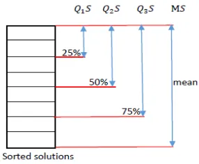
This paper uses the following training set definition strate-gies (Zhang, Zhou, and Zhang 2018), which are also illus-trated in Figure 1.

Figure 1: Training set definition strategies

• Mean fitness separation (MS):the solutions with the

ob-jective values less than the mean fitness value, are

as-signed label+1, and the others are assigned label−1.

• First quartile fitness separation (Q1S): the best25%

so-lutions are assigned label+1, and the others are assigned

label−1.

• Median fitness separation (Q2S):the best50%solutions

are assigned label +1, and the other ones are assigned

label−1.

• Third quartile fitness separation (Q3S):the best75%

so-lutions are assigned label+1, and the others are assigned

label−1.

Model Building

Fuzzy classification (Derrac, Garcia, and Herrera 2014) is a fuzzy rule-based classification model. In real world ap-plications, a large number of concepts may generally not be described precisely, and in some situations, it does not need to accurately describe the relevant concepts of things. Based on such observations, Zadeh proposed fuzzy math-ematics based on fuzzy set theory in 1965 (Zadeh 1965; Zadeh, Klir, and Yuan 1996). As one of the popular meth-ods in fuzzy mathematics field, fuzzy classification is often applied in a fuzzy environment by using precise methods to model and classify imprecise and vague data.

(3)

which is required to be constructed given the actual problem at hand.

Let

m=F class(x)

denote a fuzzy classification model for a binary

classifi-cation problem, where x is a feature vector, and m =

(m1, m2)is the membership degree vector that belongs to

the two classes.

Some commonly used fuzzy classification models are based on neural networks, K nearest neighbors (KNN), etc. (Keller, Gray, and Givens 1985; Derrac, Garcia, and Herrera 2014). This paper uses the fuzzy KNN (FKNN) to do classification, which uses the fuzzy similarity rather than the distance in original KNN to do classification (Derrac, Garcia, and Herrera 2014).

Candidate Solution Labeling and Selection

In FCPS, for each parent solutionx,M candidate solutions,

Y ={y1, y2,· · ·, yM}, are sampled. The candidate solution

with the maximal membership degree belongs to ‘promis-ing’ class is chosen.

FCPS Assisted EA

A general FCPS assisted EA is shown in Algorithm 1.

Algorithm 1:FCPS-EA Framework

// Initialization

1 Initialize the populationP ={x1, x2,· · · , xN};

// Main loop

2 whiletermination condition is not satisfieddo

// Training Set definition

3 Assign each individualx∈Pa labell∈ {+1,−1};

// Model building

4 Train a fuzzy classifier modelm=F class(x)

based on the data set{< x, l >|x∈P}; 5 foreachx∈Pdo

// Candidate solution generation

6 Sample candidate solutions

Y ={y1_,_{· · ·}_{, y}M_}_;

// Candidate solutions labeling and selection

7 Predict the membership ofy∈Y by

m=F class(y);

8 LetV ⊆Y contain candidate solutions with

maximal membership degree belongs to ‘promising’ class;

9 Randomly choosey∈V as offspringx;

// Environmental selection

10 iff(y)< f(x)then

11 Setx=y;

12 end

13 end

14 end

In each generation, FCPS-EA maintains:

• a set ofNsolutionsP ={x1, x2,· · ·, xN}, and

• their objective valuesf(x1), f(x2),· · ·, f(xN).

Some components in Algorithm 1 are explained as follows.

• Initialization:In Line 1,N solutions are uniformly and

randomly sampled fromΩto initialize the populationP.

• Stopping condition:The algorithm stops when the

num-ber of function evaluations exceeds the given maximum

numberF ESinLine 2.

• Training set definition:InLine 3, each solution in the

cur-rent population is assigned a labell ∈ {+1,−1}where

l = +1 denotes the solution is a ‘promising’ one and

l=−1denotes the solution is a ‘unpromising’ one.

• Model building: In Line 4, a fuzzy classifier is trained

based on the labeled samples.

• Candidate solution generation:InLine 6, a set ofM

can-didate solutions are sampled with a reproduction operator.

• Candidate solution labeling and selection: In Lines

7-9, the fuzzy membership degree of the candidate

solu-tions belong to ‘promising’ class is computed according to fuzzy membership function of the fuzzy classifier and the ones with maximal membership degrees are chosen out. And finally a solution is randomly selected from the ‘promising’ candidate set as the offspring solution.

• Environmental selection:InLines 10-12, the better ones

between the current and candidate solutions are selected into the next generation according to the objective func-tion values.

Experimental Study

Algorithms in Study

The proposed FCPS strategy is integrated into two state-of-the-art evolutionary optimization algorithms, i.e., the com-posite differential evolution (CoDE) (Wang, Cai, and Zhang 2011) and the hybrid estimation of distribution algorithm with cheap and expensive local search (EDA/LS) (Zhou, Sun, and Zhang 2015) to study its performance.

CoDE CoDE (Wang, Cai, and Zhang 2011) is a

multi-operator based DE. It utilizes three mutation schemes. i.e., “DE/rand/1/bin”, “DE/rand/2/bin”, and “current-to-rand/1”, along with three groups of control parameters in candidate solution generation. In each generation, three combinations of mutation and parameter are used to generate three candi-date solutions for each parent, and the one with best fitness value is chosen as the real offspring solution. The details of the algorithm are referred to (Wang, Cai, and Zhang 2011).

(4)

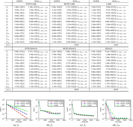
Table 1: Statistical results for the median, mean and standard deviation values of the results obtained by CoDE, EDA/LS, and

their variants onf1-f13after300,000FES over30independent runs.

median meanstd median meanstd median meanstd

FCPS-CoDE BCPS-CoDE CoDE

f1 1.86e-145[1] 1.30e-143[1]3.04e−143 5.69e-104[2] 1.37e-102[2](-)4.19e−102 2.02e-67[3] 4.88e-67[3](-)7.01e−67 f2 4.83e-77[1] 1.64e-76[1]2.55e−76 2.41e-53[2] 3.93e-53[2](-)5.47e−53 1.44e-35[3] 2.53e-35[3](-)4.15e−35 f3 9.84e-36[1] 5.84e-34[1]1.76e−33 9.16e-26[2] 9.14e-25[2](-)2.03e−24 7.13e-17[3] 9.63e-16[3](-)4.53e−15 f4 8.86e-29[1] 4.53e-27[1]1.43e−26 2.51e-23[2] 1.51e-22[2](-)4.25e−22 5.37e-16[3] 8.89e-16[3](-)9.94e−16 f5 8.69e-06[3] 2.66e-01[3]1.01e+00 7.83e-24[1] 2.39e-01[2](+)9.56e−01 5.54e-13[2] 7.97e-02[1](+)5.64e−01 f6 0.00e+00[1] 0.00e+00[1]0.00e+00 0.00e+00[1] 0.00e+00[1](∼)0.00e+00 0.00e+00[1] 0.00e+00[1](∼)0.00e+00 f7 1.62e-03[1] 1.81e-03[1]7.43e−04 1.97e-03[2] 2.14e-03[2](-)7.93e−04 2.94e-03[3] 2.84e-03[3](-)9.36e−04 f8 0.00e+00[1] 6.71e+01[3]1.06e+02 0.00e+00[1] 4.74e+00[2](∼)2.34e+01 0.00e+00[1] 2.37e+00[1](∼)1.67e+01 f9 1.99e+00[3] 2.22e+00[3]1.40e+00 0.00e+00[1] 5.97e-01[2](+)7.52e−01 0.00e+00[1] 0.00e+00[1](+)0.00e+00 f10 4.44e-15[1] 4.44e-15[1]0.00e+00 4.44e-15[1] 4.44e-15[1](∼)0.00e+00 4.44e-15[1] 4.44e-15[1](∼)0.00e+00 f11 0.00e+00[1] 1.31e-03[3]4.79e−03 0.00e+00[1] 7.39e-04[2](∼)2.69e−03 0.00e+00[1] 1.97e-04[1](∼)1.39e−03 f12 1.57e-32[1] 1.57e-32[1]5.53e−48 1.57e-32[1] 1.57e-32[1](∼)5.53e−48 1.57e-32[1] 2.07e-03[3](∼)1.47e−02 f13 1.35e-32[1] 3.66e-04[3]2.01e−03 1.35e-32[1] 2.20e-04[2](∼)1.55e−03 1.35e-32[1] 1.35e-32[1](∼)1.11e−47

+/-/∼ 2/5/6 2/5/6

FCPS-EDA/LS BCPS-EDA/LS EDA/LS

f1 3.09e-153[1] 5.57e-153[1]6.59e−153 2.26e-140[2] 3.08e-139[2](-)1.90e−138 3.59e-130[3] 5.63e-130[3](-)7.39e−130 f2 5.47e-81[1] 6.48e-81[1]4.87e−81 5.58e-70[2] 7.65e-70[2](-)6.72e−70 9.54e-65[3] 1.08e-64[3](-)7.42e−65 f3 9.25e-38[1] 1.08e-35[1]3.10e−35 1.73e-37[2] 1.17e-34[3](∼)6.18e−34 3.70e-37[3] 1.96e-35[2](∼)6.41e−35 f4 9.95e-47[1] 1.31e-46[1]9.62e−47 3.44e-45[2] 1.12e-39[3](-)7.91e−39 2.01e-42[3] 3.99e-40[2](-)2.80e−39 f5 1.94e-29[3] 1.33e-01[3]7.28e−01 1.12e-29[1] 2.27e-29[1](∼)3.07e−29 1.74e-29[2] 2.48e-29[2](∼)2.97e−29 f6 0.00e+00[1] 0.00e+00[1]0.00e+00 0.00e+00[1] 0.00e+00[1](∼)0.00e+00 0.00e+00[1] 0.00e+00[1](∼)0.00e+00 f7 2.03e-03[1] 2.13e-03[1]5.50e−04 2.22e-03[3] 2.24e-03[2](-)5.95e−04 2.19e-03[2] 2.27e-03[3](-)6.18e−04 f8 0.00e+00[1] 0.00e+00[1]0.00e+00 0.00e+00[1] 0.00e+00[1](∼)0.00e+00 0.00e+00[1] 0.00e+00[1](∼)0.00e+00 f9 0.00e+00[1] 0.00e+00[1]0.00e+00 0.00e+00[1] 1.99e-02[3](∼)1.41e−01 0.00e+00[1] 0.00e+00[1](∼)0.00e+00 f10 4.44e-15[1] 4.44e-15[1]0.00e+00 4.44e-15[1] 4.44e-15[1](∼)0.00e+00 4.44e-15[1] 4.44e-15[1](∼)0.00e+00 f11 0.00e+00[1] 3.29e-04[3]1.80e−03 0.00e+00[1] 0.00e+00[1](∼)0.00e+00 0.00e+00[1] 0.00e+00[1](∼)0.00e+00 f12 1.57e-32[1] 1.57e-32[1]5.53e−48 1.57e-32[1] 1.57e-32[1](∼)5.53e−48 1.57e-32[1] 1.57e-32[1](∼)5.53e−48 f13 1.35e-32[1] 1.35e-32[1]1.11e−47 1.35e-32[1] 1.35e-32[1](∼)1.11e−47 1.35e-32[1] 1.35e-32[1](∼)1.11e−47

+/-/∼ 0/4/9 0/4/9

0 1000 2000 3000 4000 10−150

10−100 10−50 100

1050

FES(x90)

mean f

FCPS−CoDE BCPS−CoDE CoDE

(a)f1

0 1000 2000 3000 4000 10−5

100 105

1010

FES(x90)

mean f

(b)f5

0 1000 2000 3000 4000 10−4

10−2 100 102 104

FES(x90)

mean f

(c)f7

0 1000 2000 3000 4000 10−15

10−10 10−5 100

105

FES(x90)

mean f

(d)f10

Figure 2: The mean function value of the best individuals obtained by CoDE and its variants versus FES on 4 instances over 30 independent runs.

1e−10 1e−20 1e−30 1e−40 1e−50 1e−60 1e−70 0

2 4 6 8 10 12 14 16

18x 10

4

FCPS−EDA/LS BCPS−EDA/LS EDA/LS

(a)f1

1e−05 1e−10 1e−15 1e−20 1e−25

0 1 2 3 4 5 6 7 8

9x 10

4

(b)f5

1 1e−01 1e−02

0 0.5 1 1.5 2

2.5x 10

4

(c)f7

1 1e−05 1e−10

0 1 2 3 4 5

6x 10

4

(d)f10

(5)

Experimental Settings

The first 13 benchmark functions from the YLL test suite (Yao, Liu, and Lin 1999) are employed for empirical

study. Among the test problems,f1-f4 are unimodal,f5 is

unimodal whenn= 2andn= 3, and is multimodal when

n > 3, f6 is a step function, f7 is with white noise, and

f8-f13 are multimodal. All the test instances have an

opti-mal objective value0. The definitions of these functions are

referred to (Yao, Liu, and Lin 1999).

The variable dimensions aren= 30for all instances. The

population size isN = 150for EDA/LS and its variants, and

N = 30for CoDE and its variants. The stop condition is

fit-ness evaluations (FES) = 300,000 for all of the algorithms.

Each algorithm is executed on each test instance for30

in-dependent runs. For FCPS based approaches, the number of

candidate solutions isM = 4. The other control parameters

are the same as in the original algorithms (Zhou, Sun, and Zhang 2015; Wang, Cai, and Zhang 2011).

In the experiments, FCPS is also compared with BCPS. As suggested in (Zhang, Zhou, and Zhang 2018), the classi-fication and regression trees (CART) based BCPS approach performs best than other binary classification models, be-sides K nearest neighbor (KNN). Thus, in this paper in order to evidence the efficiency of FCPS model, the CART model

is employed. TheMSstrategy is used for training set

defini-tion.

In the following subsections, CoDE and EDA/LS, their variants with FCPS, i.e., FCPS-CoDE and FCPS-EDA/LS, and their variants with BCPS (Zhang, Zhou, and Zhang 2018), i.e., BCPS-CoDE and BCPS-EDA/LS, are empiri-cally studied.

The Wilcoxon rank sum test is used to compare the

ex-perimental results, where “+”, “−”, or “∼” in the tables

in-dicate the value obtained by an algorithm is smaller than, greater than, or similar to that obtained by its FCPS based

version at95%significance level. The value in the brackets

denote the corresponding rank value in the tables.

Experimental Results

Table 1 summarizes the median, mean and standard devia-tion of the results obtained by CoDE, EDA/LS and their vari-ants on the 13 YLL test instances after 300,000 FES over 30 runs respectively. Table 2 records the rank values obtained by the algorithms. The experimental results are summarized as follows.

CoDE and its variants: The results in Table 1 suggest

that onf1-f4,f7, FCPS-CoDE performs better than CoDE;

on f6, and f8,f10−f13, the two algorithms obtain

sim-ilar results; and on f5, f9, FCPS-CoDE performs worse

than CoDE. Onf1 −f4,f7, FCPS-CoDE performs better

than BCPS-CoDE; onf5andf9, BCPS-CoDE outperforms

FCPS-CoDE; and on other 6 instances, the two algorithms obtain similar results.

EDA/LS and its variants: The results in Table 1 suggest

that on f3, f5,f6, and f8 −f13, FCPS-EDA/LS,

BCPS-EDA/LS, and EDA/LS obtain similar results; and onf1,f2,

f4,f7, FCPS-EDA/LS gets the best results.

The Wilcoxon rank sum test also shows that on most of the instances, the FCPS variant works no worse than the

original algorithms and the corresponding BCPS variants. The rank values in Table 2 also suggest that according to

Table 2: Statistical results of rank values in Table 1.

median mean

Rank 1 2 3 mean 1 2 3 mean

FCPS-CoDE 11 0 2 1.31 8 0 5 1.77

BCPS-CoDE 8 5 0 1.38 3 10 0 1.77

CoDE 7 1 5 1.85 7 0 6 1.92

FCPS-EDA/LS 12 0 1 1.15 11 0 2 1.31

BCPS-EDA/LS 8 4 1 1.46 7 3 3 1.69

EDA/LS 7 2 4 1.77 7 3 3 1.69

both the median value and the mean value, the FCPS vari-ants of CoDE and EDA/LS always achieve the best mean rank values.

Figure 2 plots the run time performance of FCPS-CoDE, BCPS-CoDE and CoDE on four test instances. It shows that

onf1,f7,f10FCPS-CoDE in red curve converges faster than

BCPS-CoDE and CoDE. Onf5BCPS-CoDE is the fastest

one.

Figure 3 plots the median FES obtained by FCPS-EDA/LS, BCPS-EDA/LS and EDA/LS when achieve the

same values on four representative test instances f1, f5,

f7, f10. The figure suggests on all of the test instances

FCPS-EDA/LS always uses the smallest numbers of FES to achieve the fitness values.

The above results indicate that the FCPS assisted ap-proaches work no worse than the original algorithms and the BCPS based approaches on most of the 13 test instances. This also suggests that FCPS could be regarded as a general strategy to improve the performances of existing EAs.

Influence of Training Set Definition Strategies

This section studies the 4 training data set definition strate-gies. In this study, CoDE is chosen as the basic optimizer in the experiments.

The statistical results for FCPS-CoDE with the 4 training set definition strategies on 4 test instances after 300,000 FEs over 30 independent runs are shown in Figure 4.

Figure 4 shows FCPS-CoDE with Q1S, Q2S, and Q3S

perform similarly and are worse than FCPS-CoDE with MS. This suggests that the population can be stably partitioned into two classes by the mean objective value of the current population. The reason might be that MS is statistically more stable than the other three strategies. To this end, the MS strategy might be a promising choice.

Comparison between FCPS and BCPS Strategies

(6)

0 1 2 3

x 105 10−150

10−100 10−50

100

1050

FES

mean f

MS Q₁S

Q2S Q₃S

(a)f1

0 1 2 3

x 105 10−30

10−20 10−10

100

1010

FES

mean f

MS Q₁S

Q2S Q₃S

(b)f4

0 1 2 3

x 105 100

101 102

103

FES

mean f

MS Q₁S

Q2S Q₃S

(c)f9

0 2 4 6

x 104 10−10

10−5 100

105

FES

mean f

MS Q₁S

Q2S Q₃S

(d)f11

Figure 4: The run time performance of FCPS-CoDE with 4 training set definition strategies on 4 instances over 30 independent runs.

Table 3: The median, mean, max, min of win numbers obtained by FKNN-CoDE comparing to those of CART-CoDE in each generation.

f1 f2 f3 f4 f5 f6 f7 f8 f9 f10 f11 f12 f13

mean 22 22 21 21 26 20 15 20 20 25 20 20 29

median 22 22 21 21 30 20 15 20 20 25 20 20 30

max 30 29 29 29 30 28 25 29 30 30 29 29 30

min 11 12 11 11 12 10 5 10 10 10 10 10 12

win generations 9971 9967 9914 9950 9960 9830 5998 9841 9805 9995 9799 9715 9990

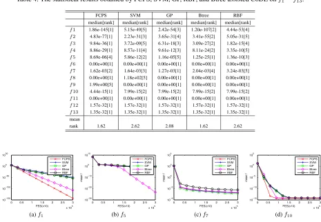
Table 4: The statistical results obtained by FCPS, SVM, GP, RBF, and Btree assisted CoDE onf1−f13.

FCPS SVM GP Btree RBF

median[rank] median[rank] median[rank] median[rank] median[rank]

f1 1.86e-145[1] 5.15e-49[5] 2.42e-54[3] 1.20e-107[2] 4.44e-53[4] f2 4.83e-77[1] 2.23e-31[3] 3.65e-31[4] 3.41e-55[2] 5.05e-31[5] f3 9.84e-36[1] 3.72e-09[5] 6.31e-18[3] 3.09e-27[2] 1.82e-15[4] f4 8.86e-29[1] 8.57e-11[4] 9.61e-12[3] 8.11e-24[2] 3.35e-10[5] f5 8.69e-06[4] 5.86e-12[2] 1.16e-05[5] 1.25e-25[1] 1.36e-10[3] f6 0.00e+00[1] 0.00e+00[1] 0.00e+00[1] 0.00e+00[1] 0.00e+00[1] f7 1.62e-03[2] 1.64e-03[3] 1.27e-03[1] 2.04e-03[4] 3.24e-03[5] f8 0.00e+00[1] 1.18e+02[5] 0.00e+00[1] 0.00e+00[1] 0.00e+00[1] f9 1.99e+00[5] 0.00e+00[1] 0.00e+00[1] 0.00e+00[1] 0.00e+00[1] f10 4.44e-15[1] 7.99e-15[2] 7.99e-15[2] 7.99e-15[2] 7.99e-15[2] f11 0.00e+00[1] 0.00e+00[1] 0.00e+00[1] 0.00e+00[1] 0.00e+00[1] f12 1.57e-32[1] 1.57e-32[1] 1.57e-32[1] 1.57e-32[1] 1.57e-32[1] f13 1.35e-32[1] 1.35e-32[1] 1.35e-32[1] 1.35e-32[1] 1.35e-32[1] mean

rank 1.62 2.62 2.08 1.62 2.62

0 0.5 1 1.5 2 2.5 3

x 105 10−150

10−100 10−50 100 1050

FES(x10)

mean f

(a)f1

0 0.5 1 1.5 2 2.5 3

x 105 10−30

10−20 10−10 100 1010

FES(x10)

mean f

(b)f5

0 0.5 1 1.5 2 2.5 3

x 105 10−4

10−2 100 102 104

FES(x10)

mean f

(c)f7

0 0.5 1 1.5 2 2.5 3

x 105 10−15

10−10 10−5 100 105

FES(x10)

mean f

(d)f10

(7)

Table 5: The median, mean, max, min of win numbers obtained by FKNN-CoDE comparing to those of Btree-CoDE in each generation.

f1 f2 f3 f4 f5 f6 f7 f8 f9 f10 f11 f12 f13

mean 22 23 22 23 26 18 16 19 19 24 19 19 29

median 22 23 22 22 26 18 15 19 19 24 19 18 30

max 30 30 30 29 30 28 25 29 29 30 28 29 30

min 10 11 12 11 12 8 5 7 6 13 8 8 14

win generations 9934 9984 9986 9973 9983 9249 5807 9252 9323 9995 9273 9121 9996

is recorded 1_{. This comparison is applied to each}

genera-tion. The test instances f1−f13 are chosen for empirical

study. CoDE is chosen as the basic optimizer in the

exper-iments. The population size is30. The experimental results

are shown in Table 3.

From Table 3, it can be seen that16.67%-100.00%

off-spring solutions chosen by the FKNN model are better than those chosen by the CART model, and on the contrary, only

0.00%-83.33% offspring solutions chosen by the CART model are better than those chosen by the FKNN model. The median and mean values are quite consistent. According to

the mean values,50%-96.67%offspring solutions chosen by

the FKNN model are better than those chosen by the CART

model. It is clear that except f7, in over97%generations,

more than50.00%offspring solutions chosen by the FKNN

model are better than those chosen by the CART model on all the other test instances. This suggests that the FKNN per-forms better than CART on choosing offspring solutions.

Comparison between Fuzzy Classification and

Surrogate Models

This section compares FCPS and surrogate model based pre-selection (SPS) assisted CoDE. The surrogate model em-ployed in this section are SVM, GP, Btree, RBF. For sim-plicity, the name of the model is directly used to represent CoDE with the corresponding strategy.

Table 4 summarizes the median results obtained by FCPS, SVM, GP, Btree, RBF assisted CoDE on the 13 YLL test in-stances after 300,000 FES over 30 independent runs respec-tively.

The rank values in Table 4 suggest that FCPS and Btree assisted CoDE achieve the best mean rank value.

Figure 5 plots the mean run time performance of FCPS, SVM, GP, Btree, RBF assisted CoDE on 4 test instances.

The figure presents that onf1,f10, FCPS assisted CoDE in

red curve converges faster than the others, and the Btree

assisted CoDE performs the second best. On f5 Btree

as-sisted CoDE performs the best, and on f7, GP assisted

CoDE is faster than the others, and FCPS and Btree as-sisted CoDE perform similarly. Thus it can be concluded that FCPS assisted CoDE outperforms the surrogate model assisted CoDE. And for the surrogate models, the Btree model is the best one.

In order to investigate why the fuzzy classification model works better than the surrogate model, the following experi-ment is conducted. For a given population, both FKNN and

1

The number of win solutions achieved by CART-CoDE equals to the population size minus that achieved by FKNN-CoDE.

Btree models are built, then the models are used to predict the quality of the newly generated candidate solutions, and finally an offspring solution is chosen according to each of the models. The two offspring solutions are compared ac-cording to the real function values, and the number of win

solutions achieved by the FKNN model is recorded2. This

comparison is applied to each generation. The test instances

f1−f13 are chosen to do the experiment. The population

size is30. The experimental results are shown in Table 5.

From Table 5, it can be seen that16.67%-100.00%

off-spring solutions chosen by the FKNN model are better than those chosen by the Btree model, and on the contrary, only0.00%-83.33%offspring solutions chosen by the Btree model are better than those chosen by the FKNN model. The median and mean values are quite consistent. According to

the mean values, 53.33%-96.67% offspring solutions

cho-sen by the FKNN model are better than those chocho-sen by the

Btree model. It is also clear that exceptf7, in over91.00%

generations, more than50.00%offspring solutions chosen

by the FKNN model are better than those chosen by the Btree model on all the other test instances. This suggests the FKNN performs better than Btree on choosing offspring so-lutions. It can also be concluded that FCPS can significantly improve the performance of EAs than surrogate models.

Conclusions

This paper proposed a fuzzy classification based preselec-tion (FCPS) strategy for evolupreselec-tionary optimizapreselec-tion. FCPS applies a fuzzy classification model instead of a binary clas-sification model to assist preselection. To apply FCPS in EAs, firstly a fuzzy classification model is built according to the current solutions that belong to the ’promising’ and ’un-promising’ training data sets. Then, for each parent solution, a set of candidate solutions are sampled by the variation op-erator. Finally, a solution belongs to the ‘promising’ class with maximal membership degree according to the fuzzy classification model is chosen as the offspring solution.

FCPS is applied to two state-of-the-art algorithms, i.e., CoDE (Wang, Cai, and Zhang 2011), EDA/LS (Zhou, Sun, and Zhang 2015), and studied on 13 YLL test in-stances (Yao, Liu, and Lin 1999). The CART based BCPS scheme is also employed for comparison study. The exper-imental results suggest that on most cases, the FCPS based approach works better than the BCPS based approach and the original algorithm. Some more discussions have also

2

(8)

proved that the fuzzy classification model is more efficient than the CART model and surrogate model on prediction in evolutionary optimization.

Some future work to improve the performance of FCPS-EA could be in following ways: (a) find a more proper way to combine fuzzy classification with EAs, and (b) reduce the computational cost in fuzzy classification building.

Acknowledgments

This work is supported by the National Natural Sci-ence Foundation of China (No. 61731009, 61673180, and 61703382), and the Fundamental Research Funds for the Central Universities.

References

Back, T.; Fogel, D. B.; and Michalewicz, Z. 1997.

Hand-book of Evolutionary Computation. CRC Press.

Chen, Y.; Xie, W.; and Zou, X. 2013. How can surrogates

in-fluence the convergence of evolutionary algorithms?Swarm

and Evolutionary Computation12:18–23.

Das, S., and Suganthan, P. N. 2011. Differential evolution:

A survey of the state-of-the-art. IEEE Transactions on

Evo-lutionary Computation15(1):4–31.

Derrac, J.; Garcia, S.; and Herrera, F. 2014. Fuzzy nearest neighbor algorithms: Taxonomy, experimental analysis and

prospects. Information Sciences260:98–119.

Emmerich, M.; Giotis, A.; Ozdemir, M.; Back, T.; and Gi-annakoglou, K. 2002. Metamodel-assisted evolution

strate-gies. InInternational Conference on Parallel Problem

Solv-ing from Nature (PPSN’ 02), 361–370.

Hu, Y.-Q.; Qian, H.; and Yu., Y. 2017. Sequential

classification-based optimization for direct policy search. In Proceedings of the 31st AAAI Conference on Artificial

Intel-ligence (AAAI’ 17), 2029–2035.

Jin, Y. 2003. A comprehensive survey of fitness

approxima-tion in evoluapproxima-tionary computaapproxima-tion. Soft Computing9(1):3–

12.

Jin, Y. 2011. Surrogate-assisted evolutionary computation:

Recent advances and future challenges. Swarm and

Evolu-tionary Computation1(2):61–70.

Keller, J. M.; Gray, M. R.; and Givens, J. A. 1985. A fuzzy

k-nearest neighbor algorithm. IEEE Transactions on Systems,

Man, and Cybernetics(4):580–585.

Klir, G., and Yuan, B. 1995. Fuzzy sets and fuzzy logic,

volume 4. New Jersey: Prentice hall.

Larraaga, P., and Lozano, J. A. 2001.Estimation of

Distribu-tion Algorithms: A New Tool for EvoluDistribu-tionary ComputaDistribu-tion,

volume 2. Springer Science & Business Media.

Li, Y.; Zhou, A.; and Zhang, G. 2014. An MOEA/D with

multiple differential evolution mutation operators. In

Pro-ceedings of the 2014 IEEE Congress on Evolutionary

Com-putation (CEC’ 14), 397–404.

Lu, X.-F., and Tang, K. 2012. Classification- and regression-assisted differential evolution for computationally expensive

problems. Journal of Computer Science and Technology

27(5):1024–1034.

Lu, X.; Tang, K.; and Yao, X. 2011. Classification-assisted differential evolution for computationally expensive

prob-lems. In Proceedings of the 2011 IEEE Congress on

Evo-lutionary Computation (CEC’ 11), 1986 – 1993.

Mahfoud, S. W. 1992. Crowding and preselection

revis-ited. InInternational Conference on Parallel Problem

Solv-ing From Nature (PPSN’ 92), 27–36.

Mallipeddi, R., and Suganthan, P. N. 2014. Unit commit-ment - a survey and comparison of conventional and nature

inspired algorithms. International Journal of Bio-Inspired

Computation6(2):71–90.

Polak, E. 1997. Optimization: algorithms and consistent

approximations. Springer-Verlag New York.

Qian, C.; Yu, Y.; and Zhou, Z.-H. 2015. Pareto ensemble

pruning. InProceedings of the 29th AAAI Conference on

Artificial Intelligence (AAAI’15), 2935–2941.

Szu, H. H. 1986. Non-convex optimization. InReal-Time

Signal Processing IX. International Society for Optics and

Photonics, volume 698, 59–68.

Wang, Z.; Zoghi, M.; Hutter, F.; Matheson, D.; and De Fre-itas, N. 2013. Bayesian optimization in high dimensions

via random embeddings. InProceedings of the 23rd

Inter-national Joint Conference on Artificial Intelligence (IJCAI’

13), 1778–1784.

Wang, Y.; Cai, Z.; and Zhang, Q. 2011. Differential evo-lution with composite trial vector generation strategies and

control parameters. IEEE Transactions on Evolutionary

Computation15:55–66.

Wang, H.; Qian, H.; and Yu, Y. 2018. Noisy derivative-free

optimization with value suppression. InProceedings of the

32nd AAAI Conference on Artificial Intelligence (AAAI’ 18),

1447–1454.

Yao, X.; Liu, Y.; and Lin, G. 1999. Evolutionary

program-ming made faster.IEEE Transactions on Evolutionary

Com-putation3(2):82–102.

Yu, Y.; Qian, H.; and Hu, Y.-Q. 2016. Derivative-free

opti-mization via classification. InProceedings of the 30th AAAI

Conference on Artificial Intelligence (AAAI’ 16), 2286–

2292.

Yuille, A. L., and Rangarajan, A. 2002. The concave-convex

procedure (cccp). In Advances in neural information

pro-cessing systems 14 (NIPS’01), 1033–1040.

Zadeh, L. A.; Klir, G. J.; and Yuan, B. 1996. Fuzzy sets,

fuzzy logic, and fuzzy systems: Selected papers. Advances

in Fuzzy Systems - Applications and Theory.

Zadeh, L. A. 1965. Fuzzy logic and its applications. New

York, NY, USA.

Zhang, J.; Zhou, A.; and Zhang, G. 2018. Preselection via

classification: A case study on global optimization.

Interna-tional Journal of Bio-Inspired Computation11(4):267–281.

Zhou, A.; Sun, J.; and Zhang, Q. 2015. An estimation of distribution algorithm with cheap and expensive local search

methods. IEEE Transactions on Evolutionary Computation