Certifying the True Error: Machine Learning in Coq with Verified Generalization Guarantees

(1)

The Thirty-Third AAAI Conference on Artificial Intelligence (AAAI-19)

Certifying the True Error: Machine Learning in Coq with

Verified Generalization Guarantees

Alexander Bagnall, Gordon Stewart

Ohio University, Athens, OH 45701

{ab667712, gstewart}@ohio.edu

Abstract

We present MLCERT, a novel system for doing practical mechanized proof of the generalization of learning procedures, bounding expected error in terms of training or test error. ML-CERTis mechanized in that we prove generalization bounds inside the theorem prover Coq; thus the bounds are machine checked by Coq’s proof checker. MLCERTis practical in that we extract learning procedures defined in Coq to executable code; thus procedures with proved generalization bounds can be trained and deployed in real systems. MLCERTis well documented and open source; thus we expect it to be usable even by those without Coq expertise. To validate MLCERT, which is compatible with external tools such as TensorFlow, we use it to prove generalization bounds on neural networks trained using TensorFlow on the extended MNIST data set.

1 Introduction

There is great optimism regarding the potential of artificial intelligence, and machine learning in particular, to automate tasks currently performed by humans. But there are also at-tendant challenges. In adversarial contexts, recent work at the intersection of machine learning and security has demon-strated that an attacker can exploit the sensitivity of a net-work to small input perturbations, so-called adversarial exam-ples (Szegedy et al. 2013), in order to force misclassifications with high confidence. More broadly, machine learning sys-tems can go wrong or be exploited in a variety of ways, at both training and inference time, as Papernot et al. compre-hensively survey (Papernot et al. 2016). As machine learning becomes critical infrastructure in systems like autonomous vehicles, practitioners must ensure that machine-learned com-ponents do not invalidate high-level safety and security prop-erties of the systems in which they are embedded.

In this paper, we make progress toward securing the foun-dations of machine learning practice by presenting a new system, MLCERT, for building certified implementations of learning procedures, those with machine-checked generaliza-tion guarantees in a theorem prover. With respect to related work, which is primarily SMT-based (e.g., (Katz et al. 2017)), we target deeper functional specifications such as general-ization error, or the expected error of a learned model when deployed on the distribution against which it was trained.

data set

TensorFlow

executable model

𝑒𝑟𝑟 ≤ 𝑒𝑟𝑟6 + 𝜖 prove _MLCert

Figure 1: MLCERT

Our technical approach (Figure 1) composes tools from in-teractive theorem proving, learning theory and statistics, and quantized neural networks (Hubara et al. 2016), those that learn low-precision weights. We train models either in ML-CERT, which is embedded in the Coq theorem prover (Bertot and Cast´eran 2013) or using an external tool such as Tensor-Flow (Abadi et al. 2016). We prove generalization bounds, relating expected to experimental error, using mechanized libraries of results from learning theory and statistics such as Chernoff inequalities, treating learning procedures as proba-bilistic programs with a denotational semantics in the style of (Kozen 1985). To validate experimental error of the Coq implementation of a model when run on a set of examples, we extract models to executable OCaml or Haskell code, which we then compile and run against an input data set. Statistical techniques for proving generalization are depen-dent on the complexity of the hypothesis class being learned. To tighten bounds without compromising performance, we use techniques from neural network quantization (Jacob et al. 2017) to learn accurate models with nontrivial general-ization bounds for the extended MNIST (EMNIST) digit classification task (Cohen et al. 2017).

Contributions.To summarize, the primary technical con-tributions of this paper are as follows:

• We present MLCERT (§§3 and 4), the first system for learning executable classifiers with certified generalization guarantees, bounding with mechanical proof in a theorem prover the expected error of machine-learned models.

(2)

demonstrate by proving generalization guarantees for quan-tized neural networks trained using TensorFlow (§5), for the EMNIST digit classification task (§6).

• Our implementation of MLCERTis open source online.1

Limitations. The formal generalization guarantees we prove in this paper, that expected error on an underlying distributionDis close to training or test error on a sample S drawn fromD, do not preclude adversaries that poison the training data, thus distorting our view of the underlying distributionD; or interfere with sampling, thus invalidating assumptions like independence; or shift the distribution from which examples are drawn during deployment (so-called dis-tribution drift (Papernot et al. 2016)).

Because we use statistical techniques such as Chernoff bounds, our approach also requires that training and test data are large relative to model size, which is unrealistic for models like those deep neural networks that have many more parameters than training and test examples. Our cur-rent best generalization bounds from training error for EM-NIST (Section 6) are still quite loose (77%). Our best bounds from test error on EMNIST are better (94%) but require many test examples (40k), which is unrealistic for some data sets. Nevertheless, by proving generalization bounds in Coq, we do get (probabilistic) guarantees – assuming suf-ficient training or test data – of the absence of overfitting errors. Our approach is also extensible to stochastic neural networks (Hinton and Van Camp 1993; McAllester 1999; Langford and Caruana 2002) for which researchers have recently achieved reasonably tight bounds even for large net-works (Dziugaite and Roy 2017). We plan to apply MLCERT to stochastic nets in future work.

Why Prove Generalization?Machine learning practition-ers ensure that a model generalizes by evaluating its perfor-mance on a holdout test set. Why should one care, then, whether a model isprovedto generalize? By bounding ex-pected error from training error, one no longer needs a test set, which can be useful – at least for very small model classes – when data is scarce. Using a test set also requires that one make additional independence assumptions (parameters are selected independently from the holdout set), which have been confounded by practices likep-hacking(Head et al. 2015). By certifying generalization bounds in Coq, we build proof artifacts that can be disseminated and checked with high assurance, facilitating replicable science.

From the perspective of the designer of high assurance software, generalization is useful in another way, as a natural specification of classifiers that increasingly form components of larger verified systems. For example, one might show, from bounded expected error of a neural network approxi-mating a control law, that a brake controller will with high probability apply enough force to safely brake a car. Spec-ifying and proving generalization bounds within a theorem prover facilitates the proof of end-to-end results such as these – the brake controller safely halts the car – with very high assurance. Certified generalization bounds may have appli-cation in scientific computing as well, to confirm with high

1

http://MLCert.org

assurance error bounds on, e.g., models for background noise classification in the Higgs boson LHC experiments (Baldi, Sadowski, and Whiteson 2014).

Trusted Computing Base. Our prototype currently as-sumes the following two textbook results as axioms: Pinsker’s inequality, stating that the relative entropy of two distribu-tions is bounded by a function of their total variation dis-tance; and Gibb’s inequality, stating that the relative entropy of two distributions is nonnegative. We axiomatize vector and floating point types and operations, as well as cardinality lemmas for vectors and floating point numbers. Our results also depend, as is typical of mechanized developments in the Coq theorem prover, on the correctness of tools in the Coq ecosystem such as the Coq proofchecker and Coq extraction.

2 Background

Theorem Proving.Theorem provers such as Coq (Bertot and Cast´eran 2013) enable programmers to build software and to prove its correctness all within the same programming environment. In this work, we use Coq for program proof – to validate with high assurance that implementations of learn-ing procedures generalize – but also to manage the details of proofs of mathematical theorems, such as Hoeffding’s inequality, upon which the software correctness arguments depend. Proofs in Coq proceed interactively: the programmer constructs a correctness argument in dialog with the proof management system, which displays a representation of the proof state at each point. Once the programmer completes a proof in Coq, it is checked by Coq’s proof checker, a small kernel implementing Coq’s internal dependent type theory. Correctness arguments in Coq therefore have small trusted computing bases: their correctness depends on the correct-ness of the Coq proof checker (and any assumed axioms) but not on that of the rest of the proof management system.

Learning Theory.The goal of supervised learning is to find a hypothesis h ∈ H : X → Y, for some classH mappingX’s to labelsY, that minimizes a metric like ex-pected errorE(h(x), y)(or equivalently, maximizes a met-ric like expected accuracyA(h(x), y)) when presented with a previously unseen example(x, y)drawn from a distribu-tionD. BecauseDis unknown,his learned from a training setT = [(x1, y1), . . . ,(xm, ym)]of examples, typically

as-sumed to be drawniidfromD.

A hypothesishhas lowgeneralization errorif its expected accuracyE(x,y)∼D[A(h(x), y)]is not too far from its average

empirical accuracy on training setT:

Definition 1(Generalization Error).

E(x,y)∼D[A(h(x), y)]− 1 |T|

X

(x,y)∈T

A(h(x), y)

(3)

Listing 1: Statement of Corollary 1 in Coq

Theoremchernoff :∀(:R)(eps gt0:0<), probOfR (prodRm D) [predT: training set|

letp:=learnTinexpValDAccp+ <empVal AccT p] ≤ |Params| ∗exp (−2∗2∗m).

As a reminder of one commonly used Chernoff bound, called Hoeffding’s inequality, considermiid random vari-ablesX1, . . . , Xmin the range[0,1]such that eachXi

com-putes, for instance, the accuracy of a hypothesishon sample (xi, yi)drawn from distributionD. Hoeffding’s inequality

states that the expected value ofXi(indeed, of all theXi’s –

the random variables are identically distributed) iswhpnot too much smaller than the empirical average ofX1, . . . , Xm,

assumingmis large enough. More precisely:

Theorem 1(Hoeffding’s Inequality). Givenmiidrandom variablesXi∈[0,1]overDand∈(0,1−E[X]),

Pr "

E[X] + < 1 m

X

i Xi

#

≤e−22m

For any fixed hypothesishchosen independently of a data setT, Theorem 1 gives a bound onh’s generalization error that decreases exponentially in the numbermof examples (letXiequalh’s accuracy on example(xi, yi)).2

To bound the probability thatanyhypothesish∈Hhas high generalization error, including ones learned fromT, one can combine Theorem 1 with a union bound to prove:

Corollary 1. Given a training setT ofmsamples(xi, yi) drawn iid from D and any hypothesis h (which may be learned fromT),

Pr "

E[A(h)] + < 1 m

X

i

A(h(xi), yi)) #

≤ |H|e−22m

E[A(h)] is shorthand for expected accuracy of h on an example–label pair(x, y). The right-hand side of the bound is small if the number of examplesmis large relative to|H|.3 Likewise, the probability that expected accuracy is more than less than empirical accuracy grows smaller asincreases.

Learning Theory in Coq.To make use of Theorem 1 and Corollary 1 in proofs about software, we must first translate into Coq. Listing 1 gives the Coq statement, for example, of Corollary 1. The termexpValDAccpdefines the expected accuracy of hypothesispon a sample drawn fromD, with:

DefAcc (p:Params) (i:[0, m)) (xy:X∗Y) :R:= let(x,y):=xyin ifpredictp x==ythen1else0.

2

A two-sided bound on absolute error yields right-hand side 2exp(−22m). We prove this bound in Coq but do not use it here.

3_{Corollary 1 assumes}_H_{is finite but can be applied to infinite}_H

using VC-dimension or Rademacher complexity theory, though we have not yet done so in this work. In execution settings,|H|<∞ is nearly always valid (except in symbolic algebra, implementations use fixed-width floating-point numbers). VC-dimension theory or Rademacher complexity could, however, yield tighter bounds for some hypothesis classes.

Listing 2: Generic Learners

RecordLearner (X Y Hypers Params : Type) : Type:= mkLearner{

predict : Hypers→Params→X→Y;

update : Hypers→X×Y →Params→Params}.

mapping parameterspand examples(x, y)to1or0 depend-ing on whetherpredictp xequalsy. The probability on the left-hand side of Corollary 1 is computed by the Coq function probOfR, which returns the probability, with respect to the product distributionprodRm Dofmexample–label pairs drawn fromD, of the predicate beginning[predT|. . .].

The function predict : Params→X→Y is a parameter (we instantiate it later, in§3 and§4, to particular predic-tion funcpredic-tions). The argumenti : [0, m)turns Acc into a family of functions, one for each of themsamples. Term empVal AccT pgives the empirical accuracy ofpon training setT. The hypothesispis the result of a functionlearn map-ping training sets to parameters. We elide two hypotheses in Listing 1: (1) the random variables defined by Accare mutually independent for allp, which follows from mutual independence of themsamples, and (2) expected accuracy is strictly between0and1.

3 MLC

ERT

By Example

Section 2 illustrated the translation of concentration bounds into mechanized form in Coq. Here we put the pieces together by applying these results to a case study (Perceptron).

We define learners generically (Listing 2) as pairs of func-tions:predict, which maps hyperparameters, parameters, and examplesXto labelsY; andupdate, which maps hyperpa-rameters, examples, and parameters to updated parameters of typeParams. At this level of abstraction, the functions predictandupdateand their types are all generic.

Listing 3: Linear Threshold Classifiers

Variablen: nat.(∗The dimensionality∗)

X:=float32 arrn.(∗Examples:n−arrays of floats∗)

Y:=bool.(∗Boolean labels∗)

Weights:=float32 arrn.(∗Params: weights, bias∗)

Bias:=float32.

Params : Type:=Weights×Bias.

Defpredict (p: Params) (x: X) : Y:= let(w,b):=pinf32 dotw x+b >0.

(4)

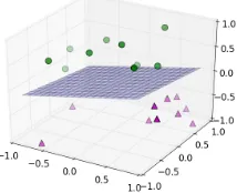
Figure 2: Model learned by certified Perceptron of Listing 4

Listing 4: Perceptron Learner (Specializes Listing 2 and Listing 3)

Variablen: nat.(∗The dimensionality∗)

Hypers:={α:float32}.(∗Learning rate∗) Defupdate (h:Hypers) (xy:(Xn)∗Y) (p:Paramsn)

: Paramsn:=

let(x,y):=xy, (w,b):=pin ifpredictp x==ythenp

else(f32 map2 (λwixi⇒wi+α∗y∗xi)w x,b+y).

DefPerceptronLearner

: Learner (Xn) Y Hypers (Paramsn):= mkLearner (λh:Hypers⇒predict) update.

Listing 4 defines a further specialization to Perceptron learning. The variablen: natagain indicates that the learner is parameterized by the dimensionality of the learning prob-lem. The new typeHypersdefines a record with a named field:αfor learning rate. The functionupdatedefines how parameterspare updated when presented with a new example (x, y). Perceptron is error driven: ifpcorrectly predictsx’s label (using the generic linear threshold prediction rule of Listing 3) thenupdatereturnspunchanged. Whenpredictp x

mispredictsy,updatereturns the new weight vector in which each weightwiequalswi+α∗y∗xi(MLCERTimplicitly co-erces the Boolean labelyto{−1,1}). The higher-order func-tionf32 map2produces a new vector component-wise from w andxaccording to the anonymous function beginning λwi xi. . . .. The overall result is a pair of the new weight

vector (defined byf32 map) and the new bias term (b+y). To execute the Perceptron learner, we use Coq to automati-cally extract it to Haskell and then compile it against a small unverified shim (also in Haskell) that produces a training set. As illustration, consider the plot of Figure 2, which depicts the model learned by our MLCERTPerceptron on random linearly separable 3-dimensional data. To generate this plot, we instrumented our Haskell shim to print both the training set and model, which we then plotted usingmatplotlib.

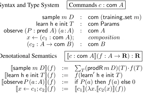
4 Generalization Bounds

In Section 3, we outlined the use of MLCERTto build a simple Perceptron learner. In this section, we demonstrate the use of MLCERTto prove – with high assurance in Coq – that the implementations of learning procedures such as Perceptron generalize to unseen examples. The core of our proof strategy is to view learning procedures as probabilistic programs in the style of (Kozen 1985) and (Gordon et al.

2014), in which a program is understood mathematically, as in the denotational semantics of Figure 3, as the expected value of a functionfover its results. To express bounds on the expected behavior of learning procedures, we use an ob-servation command,observe, to filter only those executions that satisfy a particular postcondition, such as “modelpfails to generalize”. We express generalization results as bounds on the probability mass of these filtered executions (the proba-bility of observing a nongeneralizing model should be small). Equivalently, one can think of our results as bounds on the expected value of the identity function in the subdistribution of program runs observed to produce models that fail to gen-eralize. Our semantics, like that of (Gordon et al. 2014), is naturally unnormalized due to the presence ofobserve.

Listing 5: Generic Probabilistic Learners

Defmain (D:X∗Y→R) (m:nat) (:R) (init:Params):=

T ←samplem D;(∗Drawmexamples fromD.∗) p←learn initT;(∗Learn modelp.∗)

observe(postD m )(p,T).(∗Observe postcondition.∗)

Listing 5 illustrates the general structure of probabilistic programs,main, that learn models from sampled training sets, and whose executions are then observed. The parameters ofmainare the underlying distributionD from which the training set is drawn, the number of training examplesm, and the initial parametersinit. The function first samples the training set T, then learns model pfrominit and T. The resulting modelpand training setT areobserved to satisfy a particular postcondition,post, which has the effect of filtering away those probabilistic executions that fail to satisfypost. In the context of MLCERT, we instantiatepostto:

DefpostD(m:nat) (:R) (pT:Params×training setm):= let(p, T) :=pTinexpValDAccp+ <empVal AccT p.

which, when specialized to sample sizem, distributionD, and value, yields a postcondition expressing thatpdoes not generalize well: the expected accuracy ofpis more than lower thanp’s empirical accuracy on the training setT.

To demonstrate that the probability of seeing such an exe-cution is low, we prove in Coq the following theorem:

Theoremmain bound :∀D(m >0) ( >0) (init:Params), mainD m init (λ ⇒1)≤ |Params| ∗exp (−2∗2∗m).

stating that the subdistribution of executions that satisfy post, and therefore fail to generalize, has mass less than |Params|∗exp(−2∗2_∗_m₎_{, exactly the bound of Corollary 1.} This theorem additionally assumes, as does Listing 1, the two hypotheses explained in the final paragraph of Section 2.

Holdouts.Theoremmain boundassumes that hypothesis pwas learned from the same data set on which we evaluated empirical error. Assuming access to a holdout data setnot used to learnp, we can apply MLCERTto prove tighter gen-eralization bounds that scale, by Theorem 1, asexp(−22_m₎

rather than|Params| ·exp(−22_m₎_{. To model the holdout}

(5)

Syntax and Type System Commandsc:comA samplem D : com(training setm) learn h e initT : com Params

observe(P:predA) (a:A) : comA x←(c1:comA); composition

(c2:A→comB) : comB

Denotational Semantics _Jc:comA_K(f :A→R) :R

Jsamplem DK(f) := P

T(prodRm D)(T)·f(T) Jlearn h e initTK(f) := f(learn

0_{h e init}_T₎

JobserveP(a:A)K(f) := if P(a)thenf(a)else0 Jx←c1;c2K(f) := Jc1K(λx.Jc2(x)K(f)) Figure 3: Learners: Syntax and Probabilistic Semantics

limit executions to those in which <1−expValDAccp, a precondition of Theorem 1. We then prove a theorem in Coq just likemain boundbut withmain holdouton the left-hand side and the tighter boundexp (−2∗2_∗_m₎_{on the right.}

Denotational Semantics.We give the denotational seman-tics that enables us to stateTheoremmain boundin Figure 3. The upper part of the figure defines the syntax of commands cused inmain, along with each command’s type. The nota-tionc: comAis read “cis a command with an outcome of typeA”. For example,sample(m,D) : com (training setm) is a command, parameterized by a natural numbermand dis-tributionD, that has as outcome a training set ofmexamples. Commandlearn, likewise, takes hyperparametersh, the num-ber of epochse, the initial parametersinit, and training set T and has as outcome a learned model, of typeParams. We discussedobservebriefly in the previous section: It takes a predicatePover values of typeAand valuesaof typeAand filters out executions in whichadoes not satisfyP. The final command composes commandsc1andc2in sequence, where c1has typecomAandc2has typeA→comB, notation for

a function that takes anAas argument and returns acomB

as result. The effect of sequencing is to first runc1, resulting

in an outcomexwith which we instantiate and runc2.

The lower part of the figure defines the denotational se-mantics of commands. Given a functionf mappingA’s out-comes toR, the interpretation function_Jc:comA_K(f)maps commandsctoR. Intuitively,fis a valuation function, the expected value of which we would like to compute in the distribution on outcomes generated by the interpretation of commandc. As example, consider commandsample(m,D). Its interpretation is P

T(prodRm D)(T)·f(T), exactly f’s expected value over the product distribution of m ex-amples drawn fromD. In the case ofsample,f has type training setm→R(function from training sets toR). How-ever,f’s type may differ from command to command.

As a second example, consider the interpretation of com-mand_Jobserve P a_K(f), defined asf(a)whenasatisfies predicateP and0otherwise. The effect is to remove from the support of the valuation functionf all those values a that fail to satisfyP. In the general case, in whichais pro-duced by some computationcas in the program fragment

𝑥# 𝑥$ 𝑥%&

𝑛# 𝑛$ 𝑛(

𝑜# 𝑜$ 𝑜*+,

𝑟# 𝑟$ 𝑟(

NIn

NComb

NReLU

NComb

…

shift#, scale#

𝑠ℎ𝑖𝑓𝑡#, 𝑠𝑐𝑎𝑙𝑒#

shift$, scale$

Figure 4: Structure of a network elaborated from Listing 7

Listing 6: Coq ReLU Networks

Inductivenet : Type:=

|NIn : input var→net(∗A net is (1) an input var∗)

|NReLU : net→net(∗or (2) a ReLU activation node∗)

|NComb : list (param var×net)→net.

(∗or (3) a linear combination of nets.∗)

a←c;observea P, the result is to set to0 the mass of all executions ofcproducing outcomes that do not satisfyP.

The two commands whose interpretations we have not yet discussed are learn and composition (x←c1;c2). We implementlearnby applyingf to the result of an auxiliary functionlearn0_{, which is defined as:}

Deflearn0h e (init:Params) (T:training setm) : Params:= fold (λepochpepoch⇒(∗for eachepochin[0,e):∗)

fold (λ xy p⇒(∗for eachxyinT:∗)

update hxy p))(∗update parametersp∗) pepochT) init (enum[0,e)).

The auxiliary function is implemented in the context of a learning procedure, as in Listing 2, that defines the func-tionupdate. It iterates over an outer and an inner loop (ex-pressed as functional folds), the outer of which performs the inner loopetimes, whereeis the number of epochs. The inner loop repeatedly callsupdateon eachxyexample in the training set, producing new parameterspin each iteration. We interpret command compositionx←c1;c2 as the func-tion composifunc-tion of the interpretafunc-tions ofc1andc2, namely:

Jc1K(λx.Jc2(x)K(f)). In other words, we first interpret c1, then pass its outcome, calledx, toc2(x), which is then

inter-preted with respect to the overall evaluation functionf.

5 From TensorFlow To Coq

In this section we describe our representation of neural net-work architectures in Coq as well as our net-workflow for import-ing models trained usimport-ing external tools like TensorFlow.

(6)

Listing 7: Coq Network Kernels: One Hidden Layer. Kernels are parametric in the typeTof weight parameters, the typeS of shift/scale parameters, the number of hidden nodesN, the dimensionalityINof the input space, and the numberOUT of network outputs.

DefLayer1Payload:=AxVec INT.

DefLayer1:=AxVecNLayer1Payload.

DefLayer2Payload:=AxVecN T.

DefLayer2:=AxVec OUT Layer2Payload.

Recordkernel:=

{ss1:S×S; ss2:S×S; layer1:Layer1; layer2:Layer2}.

As an example, consider the tree in Figure 4 rooted at node o1. We represent this tree as the followingnet:

x1:=NIni1;. . .;xIN:=NIniIN

n1:=NComb [(p{1,1},x1); (p{1,2},x2);. . .; (p{1,IN},xIN)],. . .

nN:=NComb [(p{N,1},x1); (p{N,2},x2);. . .; (p{N,IN},xIN)]

r1:=NReLUn1,. . .,rN:=NReLUnN

o1:=NComb [(p1,r1); (p2,r2);. . .; (pN,rN)]

in whichpvariables are parameters andivariables define inputs (neither of which are shown explicitly in Figure 4). A net with multiple outputs is a forest of inductivenets (with sharing of nodes so the forest forms a DAG). For example, the complete network of Figure 4 is represented as the forest containing as roots the nodeso1,o2,. . .,oOUT. This network

representation, while specialized to ReLU nodes, could be generalized to support other kinds of activation functions.

Kernels.The right-hand side ofmain bound(§4) scales in the cardinality of the parameter space. To represent the parameter spaces of neural networks compactly, while also facilitating cardinality proofs, we use a data structure called a kernel(Listing 7). A kernel completely determines a function in the parameter space (the space itself being fixed by the network architecture), and can be automatically elaborated to a DAG like the one in Figure 4 for execution from Coq. The kernels of Listing 7 are specialized to fully connected networks with oneN-node hidden layer (Layer1).Layer2 de-fines the network’s outputs, anOUT-length vector in which the entries, of typeLayer2Payload, areN-vectors of weights of typeT, one per hidden node. The typeAxVecsize type de-fines axiomatizedsize-vectors containing values of typetype. To import an external model to Coq, we use a Python script to generate a Coq source file containing a kernel, which can then be reasoned about in Coq and automatically extracted to OCaml or Haskell for execution.

To reduce the size of parameter spaces at the cost of a slight decrease in accuracy, we support quantization in kernels by associating with each layer a pair ofshiftandscalevalues, calledss1andss2in Listing 7 for layers 1 and 2 respectively. During elaboration to an executable net, networks with low precision weights are converted to a higher precision format, then shifted and scaled by the values for each layer. This transformation enables low precision weights to take on a wide range of possible values. The sharing of shift and scale values among weights in a layer prevents blowup in the car-dinality of the parameter space while still allowing sufficient representation flexibility. If the model being imported does

not use quantized weights, we set default values of0and1 for shift and scale respectively, to nullify their effect.

Generalization. We prove generalization of kernels in much the same way we proved generalization of Perceptron in Section 3, by bounding the mass of a probabilistic program that samples a training set, learns a network, then observes executions in which the learned classifier fails to generalize:

Variableoracle :∀m:nat, training setm→Params.

Deforacular main (D:X∗Y→R) (m:nat) (:R):=

T ←samplem D;(∗Drawmexamples fromD.∗) p←ret (oraclem T);(∗Return external modelp.∗)

observe (postD m ) (p,T).(∗Observe postcondition.∗)

The primary difference to Listing 5 is that we now assume an external learning procedure,Variableoracle, that produces models (typeParam) from training sets, modeling the training of neural networks in an external tool like TensorFlow.

Because our generalization theorems result from statistical properties of the training set and hypothesis space, we prove generalization bounds even of external training procedures, such asoracle, about which we make no assumptions.

Theoremoracular main bound :∀D(m >0) ( >0), oracular mainD m (λ⇒1)≤ |Params|∗exp(−2∗2∗m).

This bound has the same right-hand side as that of Section 4 (main bound); only the left-hand side is updated to include the oracular version ofmain. Our Coq development proves a second theorem,oracular main holdout bound, limiting gen-eralization error to the tighterexp(−2∗2∗m)when empirical error is evaluated on an independent test set. Both bounds additionally assume the two hypotheses of Listing 1, as elu-cidated at the end of Section 2.

6 Experiments

The generalization bounds of Sections 4 and 5 are most use-ful when they are reasonably tight, within a few percentage points of test error. In this section, we evaluate tightness by using TensorFlow to train two models on the EMNIST Dig-its data set (Cohen et al. 2017), which we then import into MLCERT. In our experiments, we used a fully connected network architecture with a single hidden layer consisting of 10ReLU units. We trained on a dataset of240,000examples (EMNIST’s training and validation sets) with40,000 exam-ples set aside as holdout (EMNIST’s test set). The holdout procedure, in which hypotheses are evaluated on an inde-pendent test set, yields reasonably tight bounds (∼1.5%) while the union-bound procedure, in which empirical error is evaluated as inoracular mainon the same data set on which a hypothesis was trained, yields much looser bounds, from ∼15−43%. Our best union bound results required quantiza-tion to2-bit weights, drastically decreasing the size of the parameter space but slightly decreasing accuracy.

(7)

Table 1: Experiments

W Params. Train Test Bound()

(Bits) Union Holdout

2 15,944 0.925 0.926 77%(0.152) 91%(0.016) 16 127,104 0.958 0.957 53%(0.429) 94%(0.016)

Coq source file containing the definition of a network kernel, as in Figure 7. The kernel was then elaborated to a forest in Coq, as in Figure 6, then extracted to executable code. To evaluate the accuracy of each model, we used a small unverified shim to load and feed batches of examples to the network, and to print the number of correct predictions in each batch. Then we used a Python script to compute the average number of correct predictions across all batches.

Results.Table 1 lists the accuracy of, and generalization bounds proved for, the two neural networks we trained using TensorFlow on the EMNIST data set.W is the quantiza-tion scheme: either 2-bit quantized weights or 16-bit float-ing point with no quantization. “Params.” is the size in bits of the parameter space for each network (log2|H|). “Train”

and “Test” are training- and test-set accuracy respectively. In “Bound()”, we reportat confidence1−10−9_{. To}

calcu-late “Union” bounds, we subtractfrom training error. To calculate “Holdout” bounds, we substractfrom test error.

In the “Union” case, the 2-bit quantized network has the tighter generalization bound, at0.925−0.152(=) = 77.3% expected accuracy. While the 16-bit network achieved higher training-set accuracy (0.958), its generalization bound was looser, though still nontrivial, at53%. Neither bound is very tight (for both networks, accuracy on a holdout set of40,000 examples is within a percentage point of training set accu-racy). Nevertheless, there are optimizations we have yet to perform, all of which could further tighten bounds. One is to use a sparse representation of the kernel of Figure 7 (that is, only implicitly represent the 0 weights, and use regu-larization methods like those from (Srinivas, Subramanya, and Babu 2016) to encourage0 weights during training). Another is to prove PAC-Bayes bounds for stochastic net-works (McAllester 1999), using techniques from (Dziugaite and Roy 2017) to explicitly optimize bounds during training. This would require additional work in Coq to implement and prove the correctness of sampling from stochastic nets and to extend our mechanized Chernoff bounds to PAC-Bayes.

In the “Holdout” case, we get much tighter bounds, from 91%for the 2-bit quantized network to94%for the 16-bit net-work. The value of= 0.016is the same for both networks because the holdout bound of (our mechanization of) Theo-rem 1 does not depend on model size. These bounds could likely be improved to close to1.6%of the state-of-the-art test error on EMNIST by translating into Coq a state-of-the-art network for MNIST (e.g., (Wan et al. 2013)).

From Networks to Proofs.For the networks in Table 1, our Python script automatically generates statements and proofs, as corollaries of theoremsoracular main boundand oracular main holdout boundof Section 5, of generalization

bounds specific to the network. For example, here is the “Union” bound we prove of the 2-bit network of Table 1:

Theoremtf main bound ( >0) init : tf mainDminit (λ ⇒1)≤

2ˆ(4∗16 + 784∗10∗2 + 10∗10∗2)∗exp (−2∗2∗m).

The number4∗16+784∗10∗2+10∗10∗2(15,944) is the size of the parameter space in bits. The sample sizemis240,000. Function tf mainspecializesoracular main of Section 5 to the 2-bit quantized kernel we learned using TensorFlow. As when we first presented our generic generalization bound (Listing 1), we elide two assumptions: mutual independence and the bound on the range of expected accuracy.

7 Related Work

Recent results in ML verification already span a number of points in the design space. We survey the most relevant here. Machine learning in interactive theorem provers. (Sel-sam, Liang, and Dill 2017) uses the Lean interactive the-orem prover (de Moura et al. 2015) to formally verify the correctness of programs (e.g., Auto-Encoding Variational Bayes (Kingma and Welling 2013)) for optimized sampling of stochastic computation graphs. Rather than extracting such programs to a compilable representation, as we do in ML-CERT, (Selsam, Liang, and Dill 2017) use Lean’s symbolic execution engine to interpret models interactively, executing numerically intensive tensor operations by calling out to an unverified high-performance library. (Selsam, Liang, and Dill 2017) also focus on only one particular model (stochastic computation graphs) and one particular specification (that backpropagation over computation graphs correctly com-putes gradients) while MLCERTis more general, supporting arbitrary parameter spaces and learning algorithms, and in-tegration of external tools such as TensorFlow. On the other hand, MLCERTverifies that learning procedures generalize, not that each iteration of a learning procedure correctly com-putes gradients. Thus it is possible for an MLCERTprocedure to, e.g., fail to quickly converge to low training error, while still having a tight generalization bound.

Stability analysis of probabilistic programs.We prove generalization bounds in this work by appeal to statistical results such as Chernoff bounds, which do not depend on the details of implementations of learning procedures. An alternative approach by (Barthe et al. 2017) bounds general-ization error by proving that learning procedures are stable (on only slightly different training sets, they produce only slightly different models). Because the (Barthe et al. 2017) approach reasons about properties of implementations of learning procedures, it is less easily integrated than MLCERT with external tools such as TensorFlow (one would have to prove stability of core TensorFlow libraries, including opti-mizations, a daunting task). On the other hand, proofs from stability yield bounds that are independent of the size of the parameter space, and could therefore sometimes be tighter than those achievable using Chernoff inequalities.

(8)

analysis of therobustness of neural networks: how much do model outputs differ when input examples are perturbed? Although robustness is distinct from algorithmic stability (the former applies to learned models while the latter applies to the learning process), robustness, like stability, is also deeply tied to generalization (cf. (Xu and Mannor 2012)). One goal of future work is to investigate whether the generalization bounds we prove in MLCERTcan be applied to do analysis and proof of neural network (expected) robustness.

8 Conclusion

This paper describes MLCERT, the first system for building executable machine-learned models with generalization guar-antees certified in a theorem prover. MLCERTis compatible with externally trained tools such as TensorFlow, which we use to prove nontrivial generalization guarantees for quan-tized neural networks trained on EMNIST.

Acknowledgments

We thank Razvan Bunescu, Cindy Marling, Anindya Baner-jee, and the AAAI anonymous reviewers for providing help-ful comments on an earlier draft. We also thank Samuel Merten, who mechanized a lemma, and William Kanieski, who provided a paper-and-pencil proof. This material is based upon work supported by the NSF under Grant No. CCF-1657358 and by the Ohio Federal Research Network (OFRN). Any opinions, findings, and conclusions or recommendations expressed in this material are those of the authors and do not necessarily reflect the views of the NSF or of OFRN.

References

Abadi, M.; Barham, P.; Chen, J.; Chen, Z.; Davis, A.; Dean, J.; Devin, M.; Ghemawat, S.; Irving, G.; Isard, M.; et al. 2016. Tensorflow: A system for large-scale machine learning. In OSDI, volume 16, 265–283.

Baldi, P.; Sadowski, P.; and Whiteson, D. 2014. Searching for exotic particles in high-energy physics with deep learning. Nature communications5:4308.

Barthe, G.; Espitau, T.; Gr´egoire, B.; Hsu, J.; and Strub, P.-Y. 2017. Proving expected sensitivity of probabilistic programs. Proceedings of the ACM on Prog. Lang.2(POPL):57. Bertot, Y., and Cast´eran, P. 2013.Interactive theorem proving and program development: Coq’Art: the calculus of inductive constructions. Springer Science & Business Media. Cohen, G.; Afshar, S.; Tapson, J.; and van Schaik, A. 2017. EMNIST: an extension of MNIST to handwritten letters. arXiv preprint arXiv:1702.05373.

de Moura, L.; Kong, S.; Avigad, J.; Van Doorn, F.; and von Raumer, J. 2015. The Lean theorem prover (system descrip-tion). InCADE, 378–388. Springer.

Dziugaite, G. K., and Roy, D. M. 2017. Computing nonvac-uous generalization bounds for deep (stochastic) neural net-works with many more parameters than training data.arXiv preprint arXiv:1703.11008.

Gordon, A. D.; Henzinger, T. A.; Nori, A. V.; and Rajamani, S. K. 2014. Probabilistic programming. InFuture of Software Engineering, 167–181. New York, NY, USA: ACM.

Head, M. L.; Holman, L.; Lanfear, R.; Kahn, A. T.; and Jennions, M. D. 2015. The extent and consequences of p-hacking in science.PLoS biology13(3):e1002106. Hinton, G. E., and Van Camp, D. 1993. Keeping the neural networks simple by minimizing the description length of the weights. InProceedings of the sixth annual conference on Computational Learning Theory, 5–13. ACM.

Huang, X.; Kwiatkowska, M.; Wang, S.; and Wu, M. 2017. Safety verification of deep neural networks. InInternational Conference on Computer Aided Verification, 3–29. Springer. Hubara, I.; Courbariaux, M.; Soudry, D.; El-Yaniv, R.; and Bengio, Y. 2016. Quantized neural networks: Training neural networks with low precision weights and activations.CoRR abs/1609.07061.

Jacob, B.; Kligys, S.; Chen, B.; Zhu, M.; Tang, M.; Howard, A.; Adam, H.; and Kalenichenko, D. 2017. Quantization and training of neural networks for efficient integer-arithmetic-only inference.arXiv preprint arXiv:1712.05877.

Katz, G.; Barrett, C.; Dill, D. L.; Julian, K.; and Kochen-derfer, M. J. 2017. Reluplex: An efficient smt solver for verifying deep neural networks. InInternational Conference on Computer Aided Verification, 97–117. Springer.

Kingma, D. P., and Welling, M. 2013. Auto-Encoding Varia-tional Bayes. arXiv preprint arXiv:1312.6114.

Kolter, J. Z., and Wong, E. 2017. Provable defenses against adversarial examples via the convex outer adversarial poly-tope. arXiv preprint arXiv:1711.00851.

Kozen, D. 1985. A probabilistic PDL. Journal of Computer and System Sciences30(2):162–178.

Langford, J., and Caruana, R. 2002. (Not) Bounding the True Error. InNIPS, 809–816.

McAllester, D. A. 1999. PAC-Bayesian model averaging. In Proceedings of the twelfth annual conference on Computa-tional Learning Theory, 164–170. ACM.

Papernot, N.; McDaniel, P.; Sinha, A.; and Wellman, M. 2016. Towards the science of security and privacy in machine learn-ing.arXiv preprint arXiv:1611.03814.

Paszke, A.; Gross, S.; Chintala, S.; Chanan, G.; Yang, E.; DeVito, Z.; Lin, Z.; Desmaison, A.; Antiga, L.; and Lerer, A. 2017. Automatic differentiation in PyTorch.

Selsam, D.; Liang, P.; and Dill, D. L. 2017. Developing bug-free machine learning systems with formal mathematics. In Precup, D., and Teh, Y. W., eds.,Proceedings of the 34th ICML, volume 70, 3047–3056.

Srinivas, S.; Subramanya, A.; and Babu, R. V. 2016. Training sparse neural networks.CoRRabs/1611.06694.

Szegedy, C.; Zaremba, W.; Sutskever, I.; Bruna, J.; Erhan, D.; Goodfellow, I. J.; and Fergus, R. 2013. Intriguing properties of neural networks.CoRRabs/1312.6199.

Wan, L.; Zeiler, M.; Zhang, S.; Le Cun, Y.; and Fergus, R. 2013. Regularization of neural networks using DropConnect. InICML, 1058–1066.