Term Structure of Natural Gas Futures Contracts

(1)

Term Structure of Natural Gas Futures Contracts

Guych Nuryyev

I-Shou University, Taiwan

Charles Hickson

Queen’s University Belfast, UK

ABSTRACT

This paper considers the possibility of the persistence of quasi rents in the US natural gas industry. We compare the term structure of gas and oil futures, and test for cointegration between gas and oil prices. The results indicate that natural gas yield curves are consistently higher than those of oil, reflecting possible higher risk premiums. The results also indicate that gas prices are cointegrated with and are driven by oil prices. This is consistent with the notion of oil price serving as market indicator for gas contracts with potential quasi-rents. Our findings are important in supporting the view that natural gas markets may maintain quasi-rents, despite evidence of long-term trends in improving market efficiency.

Key words: cointegration, gas futures, gas quality, hold-up, oil futures, quasi-rents, term structure, yield curve.

JEL code: Q40

Corresponding author

Guych Nuryyev: gnuriyev01@qub.ac.uk

(2)

1. INTRODUCTION AND LITERATURE REVIEW

In this paper, we explore the possibility of the existence of quasi rents in the natural gas industry stemming from hold-up costs. Over recent decades, the US natural gas industry has undergone a degree of integration, with greater degree of gas price correlations across various regions (De Vany and Walls 1993, Doane and Spulberg 1994, Serletis and Rangel-Ruiz 2004). The industry has reduced many barriers to entry, and it is widely held today to be relatively competitive (De Bock and Gijon 2011). However, natural-gas delivery generally requires very large asset-specific investments in extensive pipeline systems. Moreover, investments in such systems are undertaken after long-term market profitability projections. Consequently, natural gas traders prefer to contract longer term than, for example, oil market traders (Grout 1984). Longer term and futures contracts typically carry risk premiums (Quan 1992, Alexander 1999, Omonbude 2007, Stevens 2009).

This importance of a longer-term perspective serves as a motivation for this study. We compare risk premiums across gas futures contracts as well as with the premiums in oil futures contracts. The resulting term structure of gas futures reveals relatively high premiums, which suggest the persistence of quasi-rents in the natural gas industry. These comparisons indicate that longer-term natural gas futures contracts typically trade at a higher price than similar oil contracts, with the difference being statistically significant. They also indicate that gas futures are affected by the seasons of the year, while oil futures contracts are not so affected.

Therefore, this paper studies the relationship between gas and oil prices from the perspective of relatively high hold-up potential in natural gas industry. We test for cointegrating relationship between the futures prices of oil and natural gas. As mentioned above, traders may prefer to commit to futures contacts, even though such contacts would carry risk-premiums (Grout 1984). For this reason, longer-term comparisons between oil and natural gas market structures may be better described using futures prices rather than spot prices. Our analysis shows that natural gas and oil futures are cointegrated, although their relationship may be affected by a number of recent events in the energy market.

(3)

2011). However, our analysis shows that even with long-term cointegration, gas and oil prices can divergence over the short term.

This divergence may be due to end users’ limited ability to shift into alternative energy sources. Short-term switching between natural gas and oil typically requires significant expenditure in complementary apparatus by industrial end users. Similarly, transportation units require special engine and fuel-tank apparatus in order to be able to switch to natural gas. It is also the case for refrigeration and heating units as well as electric power plants. Moreover, in 2000, only approximately 17% of capacities of US utilities had the ability of switching between the use of petroleum liquids and natural gas, but this share decreased to approximately 14% by 2010 (EIA 2000, EIA 2010). Hence, despite the trend in freer access and the possibility of adopting sliding price mechanism, natural gas contracts could still be prone to high quasi-rents. Evidencing this is a contribution of current study.

One indirect method of extracting these quasi-rents is through indirect price discrimination based on quality of the product (Klein 1996). This paper also studies several gas quality issues, including the variability of natural gas quality, its effect on the gas prices, and indirect price discrimination based on gas quality.

The remainder of this paper is structured as follows. Section 2 presents the data used and the analysis of term structure. Section 3 presents the analysis of long-term relationship between gas and oil futures prices. Section 4 discusses the gas quality issues, and section 5 concludes this paper.

2. DATA DESCRIPTION AND TERM STRUCTURE ANALYSIS

2.1. Data description

Our analysis employs the following daily data: (i) spot and futures prices of natural gas at Henry Hub; (ii) spot and futures prices of WTI crude oil; (iii) gas energy content, carbon dioxide content, nitrogen content, and gas weight relative to that of air. Gas quality data is provided for four pipeline connections at the Henry Hub: Hub to Mainline, Mainline to Hub, Sabine – Citgo, Sabine to Calcasieu.

The data on prices pertain to the period from January 2003 until December 2010; the gas quality data pertains to the period from 01 July 2011 until 31 Oct 2011. The Energy Information Administration1_{is source of all futures prices and WTI oil spot price. The official Nebraska}

1_{The spot and futures prices are available at the following web pages (accessed on 11 Dec 2011):}

WTI spot price: http://tonto.eia.gov/dnav/pet/hist/LeafHandler.ashx?n=PET&s=RWTC&f=D

(4)

government website is source for the natural gas spot price. Sabine Pipeline Company (http://www.sabinepipeline.com) is the source of gas quality data.

2.2.Descriptive analysis of term structure of futures contracts

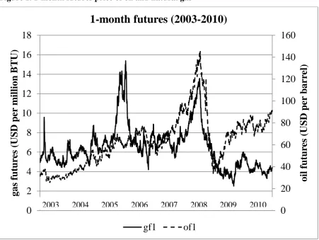
Figure 1 below compares the one-month futures price of oil with the one-month future price of natural gas. Such a graph can be useful for identifying factors impacting the relationship between the two series. In the long term, this figure suggests a stable relationship between the two price series. However, there are three distinct periods with a noticeable divergence that warrant an event study. The first episode is a spike in the gas futures price, due to reduced supply of gas caused by Hurricane Katrina, beginning in August of 2005. The second episode of note is the considerable drop in the futures prices of both commodities. This can be attributed to a negative shock for energy due to the global economic recession that began during the second half of 2008. The final apparent divergence between the two series begins around mid-2009 and it is characterised by a sharp rebound in the oil futures price. This rise is associated with a rebound in demand for energy and the launch of a large LNG receiving terminal in Louisiana. A large LNG receiving terminal can exert a downward pressure on natural gas futures prices.

Term structure of gas and oil futures contracts may reveal seasonality in the patterns of natural gas and oil prices. Term structure may also indicate if natural gas industry is prone to additional risks, as discussed in the introduction. With this motivation, yield curves for different term futures contracts for oil and gas are constructed. The available data allows yield curves with only four points on the curves – one point for each contract type. Monthly simple annualised yield is calculated for each contract based on Equation 1 and averaged across all days of the month. Although, the result of this calculation is not strictly an actual yield, the return measure can capture any arbitrage possibility, despite the fact that it ignores storage costs. For example, an investor may buy gas on the spot market and sell it on the futures market, keeping the asset until maturity provides for a return, which, in this paper, is referred to as yield for simplicity of explanations.

WTI futures price for contract 2: http://tonto.eia.gov/dnav/pet/hist/LeafHandler.ashx?n=PET&s=RCLC2&f=D

Henry Hub natural gas spot price: http://www.neo.ne.gov/statshtml/124_archive.htm

Henry Hub natural gas futures for contract 1: http://tonto.eia.gov/dnav/ng/hist/rngc1d.htm

(5)

Figure 1. 1-month futures price of oil and natural gas

gf1 – 1-month natural gas futures price of1 – 1-month crude oil futures price

Thus, we write Equation 1 as follows.

Equation 1. 𝐴𝐴𝐴𝐴𝐴𝐴𝐴𝐴𝐴𝐴𝐴𝐴𝐴𝐴𝐴𝐴𝐴𝐴𝐴𝐴𝑟𝑟𝐴𝐴𝑟𝑟𝐴𝐴𝑟𝑟𝐴𝐴= ((𝑓𝑓𝐴𝐴𝑟𝑟𝐴𝐴𝑟𝑟𝐴𝐴𝐴𝐴𝑝𝑝𝑟𝑟𝐴𝐴𝑝𝑝𝐴𝐴 − 𝐴𝐴𝑝𝑝𝑠𝑠𝑟𝑟𝑝𝑝𝑟𝑟𝐴𝐴𝑝𝑝𝐴𝐴)⁄𝐴𝐴𝑝𝑝𝑠𝑠𝑟𝑟𝑝𝑝𝑟𝑟𝐴𝐴𝑝𝑝𝐴𝐴)(12⁄𝐴𝐴) where n is the futures contract length of one, two, three or four months.

This annualised yield is somewhat similar to the convenience yield described in Brennan and Schwartz (1985), Frechette and Fackler (1999), and Ribeiro and Oliveira (2011) as an average return that a holder of a commodity receives for possibility of a shortage in the future.

In total, the analysis includes 96 pairs of oil and natural gas monthly yield curves for the period 2003 – 2010. For 60 of these pairs, all points of the yield curve of gas futures are higher than the yield curve of oil futures. In January, most of the natural gas yield curves are downward sloping. During 2003 – 2010, six out of eight yield curves in January are downwardly sloped (exception: January 2009 and 2010). In August, the gas yield curves are all upward sloping.

0

20

40

60

80

100

120

140

160

0

2

4

6

8

10

12

14

16

18 oil

fu

tu

re

s

(U

S

D

p

er

b

ar

re

l)

gas f

u

tu

re

s

(U

S

D

p

er

m

illion

B

T

U

)

1-month futures (2003-2010)

gf1

of1

(6)

The fact that most gas yield curves are higher than the oil yield curves may be explained by higher risk premiums associated with gas (Nuryyev and Chu 2014). Downward sloped gas yield curves in January and upward sloped ones in August indicate a seasonality effect. This may be explained by the expectations regarding increased consumption of electricity and heating in winter months, and reduced consumption in summer months. All of the graphs illustrating the yield curves are available upon request.

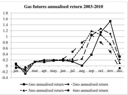
Figure 2 below illustrates the dynamics for annualised returns of gas futures over the period of a year. These dynamics are averaged over the period 2003 – 2010. In August and September the annualised returns from the futures contracts are rising, reaching levels of more than 100%. In November and December the returns are falling, and in February average annualised return is negative. As mentioned above, this is probably due to expected higher demand for gas and lower storage levels during colder months of the year.

Figure 2. Gas futures average annualised return 2003 – 2010

-0.4

-0.2

0

0.2

0.4

0.6

0.8

1

1.2

1.4

1.6

1.8 jan

feb

mar

apr may jun

jul

aug

sep

oct

nov

dec

Gas futures annualised return 2003-2010

1mo annualised return

2mo annualised return

(7)

2.3.Econometric analysis of term structure of futures contracts

As mentioned in the introduction, due to high upfront outlays and their asset specificity, corresponding natural gas contracts are prone to hold-up potential (Klein 1996). Hold-up potential increases with the length of the contract due to greater chance of a significant market change occurring. Thus, longer contracts may have higher risk premiums. In order to test if annualised return increases with contract length, we consider the spreads between the futures prices. Changes of annualised return with changes in contract length also reveal the term structure of futures contracts. Four types of spread are calculated: (1) the spread between 1-month futures and spot price, (2) the spread between 2-1-month and 1-1-month futures, (3) the spread between month and 2-month futures, and (4) the spread between 4-month and 3-month futures. Positive spreads would indicate that annualised return increases with contract length.

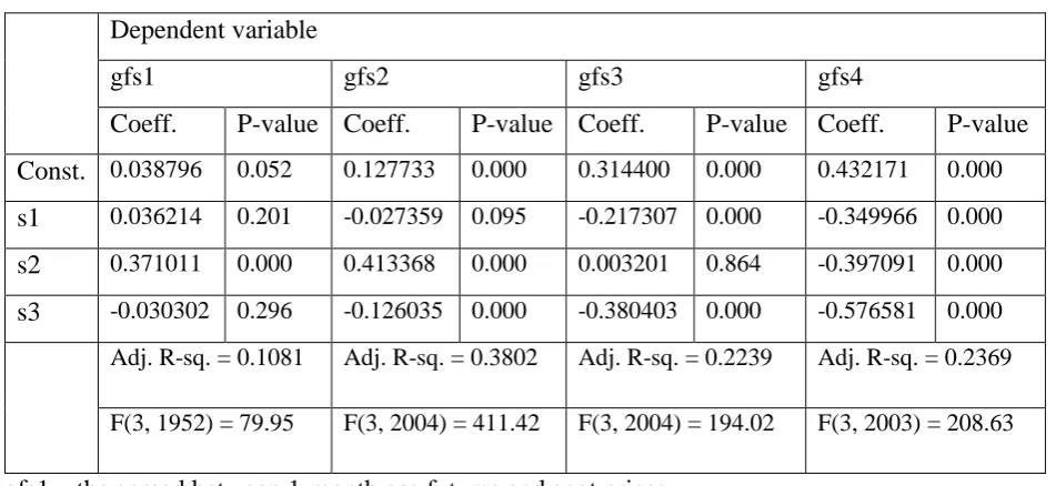
Taking into account the seasonality effect, t-test2 is used to determine whether the spreads are significantly different from zero. Table 1 below shows the results of regressing the spreads on seasonal dummy variables and a constant. This constant is employed to test whether the spreads between the futures prices are statistically significant. The term structure of natural gas futures prices over the period 2003 – 2010 is such that longer contracts have a higher gas price. This term structure is observed after having accounted for the seasonality effect. The spreads between the four futures prices are statistically significant at 1% level. The spread between the 1-month futures price and spot price is statistically significant at 10% level. This result supports the notion that longer contracts may have higher risk premiums.

The regression results also show that the gas futures spreads are affected by the seasons of the year. Generally, the spreads are smaller in spring and winter, and greater in autumn. One exception is the spread between 4-month and 3-month. This spread is greater in autumn. This may be due to the fact that in autumn the delivery date for a 4-month contract occurs during a warmer season than that for a 3-month contract. Hence, the futures price is generally higher if the delivery date is during a colder season. This implies that storage costs and capacity constraints may place the supply of gas under stress during a cold season.

2_{Unit root test (Augmented Dickey-Fuller) rejects the hypothesis of non-stationary spreads. Test results are}

(8)

Table 1. Regression of the spreads on seasonal dummy variables

Dependent variable

gfs1 gfs2 gfs3 gfs4

Coeff. P-value Coeff. P-value Coeff. P-value Coeff. P-value Const. 0.038796 0.052 0.127733 0.000 0.314400 0.000 0.432171 0.000

s1 0.036214 0.201 -0.027359 0.095 -0.217307 0.000 -0.349966 0.000

s2 0.371011 0.000 0.413368 0.000 0.003201 0.864 -0.397091 0.000

s3 -0.030302 0.296 -0.126035 0.000 -0.380403 0.000 -0.576581 0.000 Adj. R-sq. = 0.1081 Adj. R-sq. = 0.3802 Adj. R-sq. = 0.2239 Adj. R-sq. = 0.2369

F(3, 1952) = 79.95 F(3, 2004) = 411.42 F(3, 2004) = 194.02 F(3, 2003) = 208.63

gfs1 – the spread between 1-month gas futures and spot prices gfs2 – the spread between 2-month and 1-month gas futures prices gfs3 – the spread between 3-month and 2-month gas futures prices gfs4 – the spread between 4-month and 3-month gas futures prices

s1, s2, s3 – seasonal dummy variables for spring, autumn and winter respectively

Similar to the natural gas contracts, oil contracts may also incur potential hold-up costs. However, natural gas tends to be more prone to hold-up potential due to more pronounced asset specificity of investments in transportation. We examine the term structure of oil futures contracts to verifying that risk premiums of gas futures are relatively higher. Spreads between oil futures contracts were regressed on a constant and seasonal dummy variables. Similar to gas futures, oil futures prices tend to be higher for longer term contracts. However, the oil futures spreads are affected by contract length to a lesser degree. The seasonality effect of oil futures is of a different nature and of a significantly lower magnitude. In autumn, oil futures prices for longer-term contracts tend to be lower than those for shorter term contracts. This is in contrast to the behaviour of gas futures. However, the results relating to both the term structure and seasonality of oil futures are somewhat questionable, as the R-squared values of the regressions are lower than 0.033. This suggests that natural gas contracts may have relatively higher potential hold-up costs, which increase with contract duration.

A more direct comparison of natural gas and oil spreads between shorter and longer term contracts can be informative. The comparison could reveal that natural gas spreads are

(9)

higher, possibly due to higher risk premiums. In this case, the spreads between natural gas futures prices may increase faster than the corresponding spreads for oil as contract length increases. This is tested using the following technique. Firstly, the difference between the ratios of gas to oil futures of longer and shorter contracts is calculated as in Equation 2 and Equation 3. Secondly, this difference is regressed on seasonal dummy variables and a constant term. A constant that is significantly different from zero implies that gas spreads are indeed increasing faster than oil spreads.

Equation 2 𝑔𝑔𝑠𝑠𝑓𝑓𝐴𝐴1 = (𝑔𝑔𝑓𝑓1⁄𝑠𝑠𝑓𝑓1)−(𝑔𝑔𝐴𝐴𝑝𝑝 𝑠𝑠𝐴𝐴𝑝𝑝⁄ ) Equation 3 𝑔𝑔𝑠𝑠𝑓𝑓𝐴𝐴_𝑖𝑖 = (𝑔𝑔𝑓𝑓_𝑖𝑖⁄𝑠𝑠𝑓𝑓_𝑖𝑖)−(𝑔𝑔𝑓𝑓_𝑖𝑖−1⁄𝑠𝑠𝑓𝑓_𝑖𝑖−1) where i is an integer ranging from 2 to 4

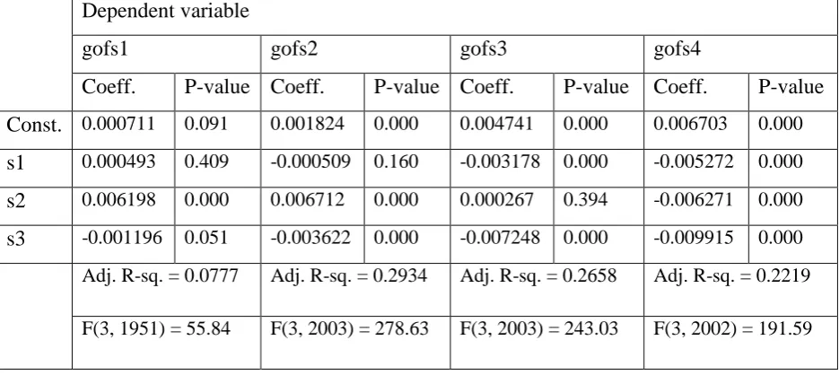
gofs1 – the difference between the ratio of 1-month gas to oil futures prices and gas to oil spot prices

gofs2 – the difference between the ratio of 2-month gas to oil futures prices and 1-month gas to oil futures prices

The next table presents the results of regressing the left-hand sides of the Equation 2 and Equation 3 on seasonal dummy variables and a constant.

Table 2. Regression of the differences between the ratios of gas to oil futures on seasonal dummy variables

Dependent variable

gofs1 gofs2 gofs3 gofs4

Coeff. P-value Coeff. P-value Coeff. P-value Coeff. P-value Const. 0.000711 0.091 0.001824 0.000 0.004741 0.000 0.006703 0.000

s1 0.000493 0.409 -0.000509 0.160 -0.003178 0.000 -0.005272 0.000

s2 0.006198 0.000 0.006712 0.000 0.000267 0.394 -0.006271 0.000

s3 -0.001196 0.051 -0.003622 0.000 -0.007248 0.000 -0.009915 0.000 Adj. R-sq. = 0.0777 Adj. R-sq. = 0.2934 Adj. R-sq. = 0.2658 Adj. R-sq. = 0.2219

(10)

The regression results show that, controlling for seasonality, the ratio of the gas to oil futures price is larger for longer contracts. This difference between contract prices is shown to be statistically significant using t-tests of the constant terms. In most cases the constants are significant at 1% level. Only the difference between the ratios of 1-month futures and spot prices is significant at 10% level. As mentioned in the introduction, this difference suggests that gas contracts are relatively more prone to quasi-rents.

3. COINTEGRATION ANALYSIS

As discussed in the introduction, natural gas and oil prices may move in tandem in the long term. However, these prices may also diverge in the short term when responding to market shocks. In order to test a long-term association of gas and oil prices, we test for cointegration between 1-month oil and natural gas futures prices. An augmented Dickey-Fuller test does not reject the null hypothesis that both the natural gas and oil futures have a unit root4. This implies that these variables may have a cointegrating relationship.

A number of dummy variables were used in the cointegration analysis. Three dummy variables control for the seasons of the year. Another three dummy variables account for the effects of hurricane Katrina, economic recession in the second half of 2008, and launch of a large receiving terminal for LNG in mid-20095. The timing of the third event approximately coincides with apparent short-term divergence between gas and oil futures6.

The cointegration analysis shows that there is a long-term relationship between oil and natural gas 1-month futures prices. Augmented Dickey-Fuller test rejects the null hypothesis of unit root of the error terms of the linear combination of the futures prices. The results of the test are shown in the Table 3 below.

Table 3. Unit root test of cointegrating vector

Dickey-Fuller test for unit root Number of obs = 1999

Test statistic 1% critical value 5% critical value 10% critical value

Z(t) -6.947 -3.430 -2.860 -2.570

MacKinnon approximate p-value for Z(t) = 0.000

4_{The results of the unit root test are available upon request.}

5_{Possible significance of the first two events is apparent. Construction of a very large LNG terminal may reduce}

regional segmentation and affect the relationship between oil and gas prices. Additionally, there is an apparent change in this relationship at approximately the same time.

6_{A similar apparent change between gas and oil spot prices was argued to illustrate decoupling by De Bock and}

(11)

Given cointegrated gas and oil futures prices, we expect gas futures to be driven by oil futures. This is because oil price often plays the role of energy market indicator for gas contracts, which have relatively higher potential hold-up costs. The remainder of this section tests whether gas futures are driven by oil futures or vice versa.

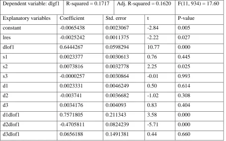
This test is implemented using an error correction model (ECM). This model also shows how oil and gas futures move back to equilibrium in their relationship after a shock. Two versions of ECMs are discussed: one with gas futures driven by oil futures, and another – vice versa. The ECMs were analysed using natural logarithmic values of the gas and oil futures prices. The results of the ECM analysis are presented in the tables below.

Table 4. ECM for gas futures being driven by oil futures

Dependent variable: dlgf1 R-squared = 0.1717 Adj. R-squared = 0.1620 F(11, 934) = 17.60

Explanatory variables Coefficient Std. error t P-value

constant -0.0065438 0.0023067 -2.84 0.005

lres -0.0025242 0.0011375 -2.22 0.027

dlof1 0.6444267 0.0598294 10.77 0.000

s1 0.0023377 0.0030613 0.76 0.445

s2 0.0073816 0.0032778 2.25 0.025

s3 -0.0000257 0.0030864 -0.01 0.993

d1 0.0023331 0.0046249 0.50 0.614

d2 -0.003741 0.0036682 -1.02 0.308

d3 0.0034176 0.004093 0.83 0.404

d1dlof1 0.7571805 0.211343 3.58 0.000

d2dlof1 -0.4705811 0.0824239 -5.71 0.000

d3dlof1 0.0656188 0.1491381 0.44 0.660

Table 5. ECM for oil futures being driven by gas futures

Dependent variable: dlof1 R-squared = 0. 1361 Adj. R-squared = 0.1250 F(11, 854) = 12.23

Explanatory variables Coefficient Std. error t P-value

constant 0.0005845 0.0022434 0.26 0.795

lres1 -0.0001837 0.0006662 -0.28 0.783

dlgf1 0.1604397 0.0255446 6.28 0.000

s1 0.0028089 0.0020704 1.36 0.175

s2 -0.0016631 0.0021217 -0.78 0.433

(12)

d1 -0.0013084 0.0028962 -0.45 0.652

d2 -0.0022285 0.0020944 -1.06 0.288

d3 0.0002513 0.0025791 0.10 0.922

d1dlgf1 0.0474914 0.0629884 0.75 0.451

d2dlgf1 0.2384254 0.0538598 4.43 0.000

d3dlgf1 -0.3679776 0.071412 -5.15 0.000

dlgf1 – first difference of natural logarithmic value of gas futures price dlof1 – first difference of natural logarithmic value of oil futures price lres/lres1 – natural logarithmic value of the lagged residual (ECM variable) d1 – dummy for the time of the Katrina hurricane

d2 – dummy for the global economic recession (starting from July 2008)

d3 – dummy for launching of a large LNG receiving terminal in Louisiana (22 June 2009) d1dlgf1/d2dlgf1/d3dlgf1 – multiplication of d1/d2/d3 and dlgf1

d1dlof1/d2dlof1/d3dlof1 – multiplication of d1/d2/d3 and dlof1

The ECMs above indicate that oil and natural gas futures prices return to their long-term equilibrium after a shock. In the ECM with gas futures driven by oil futures, the error correction equals -0.25% of the divergence from their long-term equilibrium every day. This value is statistically significant at 5% level. In the ECM with oil futures driven by gas futures, the error correction equals -0.02% every day. The latter value is statistically insignificant. This suggests that natural gas futures prices are driven by oil futures prices. This agrees with the hypothesis that the natural gas contract price may be influenced by oil price trends, the latter signalling changes in the energy market.

In the ECM with gas futures driven by oil futures, only the autumn seasonality dummy is statistically significant at 5% level. In autumn, 1-month gas futures price is 7.4% higher than in summer. This may be due to expectations of higher gas consumption and lower storage levels in the coming winter.

A change of 10% in the oil futures price leads to a 6.4% change in the natural gas futures price. This is when the effects of the recession, new LNG terminal, and the hurricane are excluded. This effect of the oil futures price is significant at 1% level.

(13)

response to a 10% change in oil futures. The hurricane’s effect on the relationship between oil and gas futures is statistically significant at 1% level. The recession decreased the responsiveness of gas futures to changes in oil futures by 4.7% for every 10% change in oil futures. This effect of the recession is statistically significant at 1% level.

4. GAS QUALITY ISSUES

The following aspects of the role of gas quality in the natural gas futures market are considered in this section. Firstly, natural gas prices might be directly affected by gas quality (Hekkert, Hendriks et al. 2005). Secondly, market information asymmetry regarding product quality can give rise to a “lemons problem” (Akelrof 1970), which may be ameliorated by quality control measures. Quality control is largely based on requirements set by pipeline companies (Foss 2004). According to contract specification of Henry Hub gas futures, gas quality meets the specifications set forth by Sabine Pipeline Company and approved by the Federal Energy Regulatory Commission (FERC). However, even with this quality control in place, gas quality variations may be considerable, especially with spot LNG deliveries from various parts of the world since mid-1990s (EIA 2012)7. Therefore, in this section we test for an effect of gas quality on spot and futures price of natural gas.

Due to non-stationary spot and futures price levels, the first differences of the price levels are used in the regressions. The Augmented Dickey-Fuller test rejects the null hypothesis of unit root for the first differences of spot and futures prices8. The variables relating to gas quality are also stationary. The regression results in the table below employ the gas quality data on the connection Henry Hub to Mainline. Similar regression results are obtained for other pipelines connected to the Henry Hub.

Table 6 below shows that the gas spot price has a positive and statistically significant effect on the gas futures price. None of the gas quality variables affects either spot or futures prices. One implication of this is that the quality control in place is adequate. However, in case of significant gas quality variations across pipelines, absence of the effect of gas quality on price may imply indirect price discrimination.

7_{In 1995, Algeria was the only source of LNG imports in the USA, by 2010 the number of LNG source-countries}

increased to seven.

(14)

Table 6. Regression of natural gas spot and futures prices on gas quality at Hub to Mainline

Dependant variable

dngsp dngf1

Coefficient P-value Coefficient P-value

constant 4.848184 0.839 -0.9693641 0.972

dngsp 0.3976749 0.009

Btu -0.0213044 0.895 0.0170734 0.927

CO2 -0.5043043 0.902 0.4411281 0.926

Grvty 30.22856 0.905 -29.3839 0.920

N2 -0.2818977 0.916 0.3251623 0.916

Adj. R-squared = 0.0434 Adj. R-squared = 0.0482

F(4, 61) = 0.32 F(5, 60) = 1.66

dngsp – first difference of natural gas spot price

dhgf1 – first difference of natural gas 1-month futures price Btu – energy content of natural gas

CO2 – carbon dioxide content of gas N2 – nitrogen content of natural gas

Grvty – weight of natural gas relative to that of air

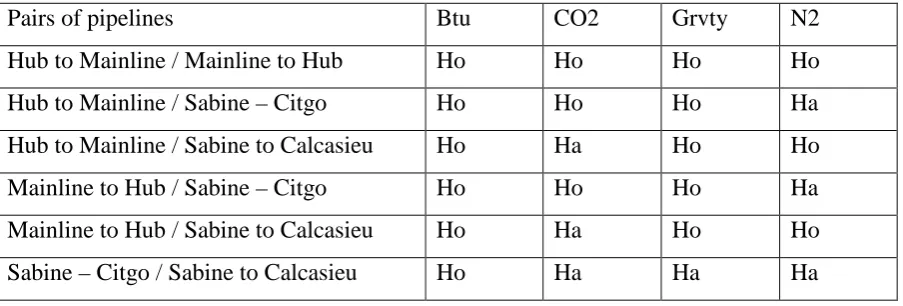
Indirect price discrimination may result from supplying gas of different quality to different pipeline destinations for the same price at the hub. To check for possible price discrimination, the gas quality data is tested for a difference in means across different pipelines to and from Henry Hub. This test is performed for all gas quality measures. The test results are available upon request. A summary of these results is provided in the Table 7 below.

(15)

Table 7. Difference in means of gas quality between pairs of pipelines

Pairs of pipelines Btu CO2 Grvty N2

Hub to Mainline / Mainline to Hub Ho Ho Ho Ho

Hub to Mainline / Sabine – Citgo Ho Ho Ho Ha

Hub to Mainline / Sabine to Calcasieu Ho Ha Ho Ho

Mainline to Hub / Sabine – Citgo Ho Ho Ho Ha

Mainline to Hub / Sabine to Calcasieu Ho Ha Ho Ho

Sabine – Citgo / Sabine to Calcasieu Ho Ha Ha Ha

Ho – The difference in means of gas quality measurements is insignificant Ha – The difference in means of gas measurements is significant

5. CONCLUSION

The main contribution of the this study is in evidencing that natural gas markets maintain quasi-rents, despite long-term trends in improving market efficiency. Natural gas industry is prone to relatively high hold-up potential, even compared to oil industry. This is due to large asset specific upfront investments and limited alternatives for transportation of gas, as well as for switching to other fuels. The potential for hold-up may leads to oil price serving as a market indicator for natural gas contracts. This, together with some level of long-term substitutability between oil and gas, can cause oil and gas prices to maintain a long-term relationship. Additionally, oil price would drive this relationship if it serves as a market indicator.

In order to test for relatively high hold-up potential, this paper compares the term structure of natural gas futures contracts with those of oil futures. For the same purpose, this paper also analyses the difference between longer and shorter futures contracts for natural gas and oil. The results demonstrate that natural gas futures contracts bear higher risk premiums than oil futures, which supports the notion of higher hold-up potential. In order to test for a long-term relationship between oil and gas futures prices, this paper conducts a cointegration analysis, followed by an error correction model. The results indicate that 1-month oil and gas futures are cointegrated. As expected, the error correction model suggests that gas futures are driven by oil futures.

(16)

the futures prices up in autumn. The model accounts for the effects of hurricane Katrina, recent recession, and new LNG terminal on the relationship between oil and gas futures. The hurricane temporarily increased the responsiveness of gas futures to changes in oil futures, while the recession decreased it. The launch of a new LNG terminal does not seem to significantly affect the relationship between gas and oil futures.

A brief analysis of gas quality shows that the effect of gas quality on the spot and futures price of natural gas is insignificant. Additionally, there is not much gas quality variations across pipelines connected to the Henry Hub, suggesting no quality-based price discrimination.

REFERENCES

Akelrof, G. A. (1970). "The market for "lemons": quality uncertainty and the market mechanism." Quarterly Journal of Economics 84: 488-500.

Alexander, C. (1999). Correlation and cointegration in energy markets. Managing Energy Price Risk, RISK Publications. 2nd edition: 291-304.

Asche, F., P. Osmundsen and M. Sandsmark (2006). "The UK market for natural gas, oil and electricity: are prices decoupled?" The Energy Journal 27: 27-40.

Bachmeier, L. and J. Griffin (2006). "Testing for market integration: crude oil, coal and natural gas." The Energy Journal 27: 55-72.

Brennan, M. J. and E. S. Schwartz (1985). "Evaluating natural resource investments." The Journal of Business 58: 135-157.

De Bock, R. and J. Gijon (2011). "Will natural gas prices decouple from oil prices across the pond?" IMF Working Paper http://www.imf.org/external/pubs/ft/wp/2011/wp11143.pdf. De Vany, A. and W. D. Walls (1993). "Pipeline access and market integration in the natural gas industry: evidence from cointegration tests." Energy Journal 14.

Doane, M. J. and D. F. Spulberg (1994). "Open access and the evolution of the U. S. spot market for natural gas." Journal of Law and Economics 37: 477-517.

EIA (2000). Inventory of electric utility power plants in the United States 2000. Washington, Energy Information Administration. http://www.eia.gov/FTPROOT/electricity/009500.pdf. EIA (2010). Electric power annual 2010. Washington, Energy Information Administration. http://www.eia.gov/electricity/annual/pdf/epa.pdf.

(17)

Foss, M. M. (2004). Interstate natural gas - quality specifications and interchangeability, Center for energy economics.

Frechette, D. L. and P. L. Fackler (1999). "What causes commodity price backwardation?" American Journal of Agricultural Economics 81: 761-771.

Grout, P. A. (1984). "Investment and wages in the absence of binding contracts: a Nash bargaining approach." Econometrica 52: 449-460.

Hekkert, M. P., F. H. J. F. Hendriks, A. P. C. Faaij and M. L. Neelis (2005). "Natural gas as an alternative to crude oil in automotive fuel chains well-to-wheel analysis and transition strategy development." Energy Policy 33: 579-594.

Klein, B. (1996). "Why hold-ups occur: the self-enforcing range of contractual relationship." Economic Inquiry 34: 444-463.

Nuriyev, G. (2011). Economics of segmented natural gas market. PhD, Queen's University Belfast.

Nuryyev, G. and H.-N. R. Chu (2014). "Effect of hold-up potential on natural gas exports." Journal of Economics and Development Studies 2(2): 191-212.

Omonbude, E. (2007). "The transit oil and gas pipeline and the role of bargaining: a non-technical discussion." Energy Policy 35: 6188-6194.

Panagiotidis, T. and E. Rutledge (2007). "Oil and gas markets in the UK: evidence from a cointegrating approach." Energy Economics 29: 329-347.

Quan, J. (1992). "Two-step testing procedure for price discovery role of futures prices." The Journal of Futures Markets 12: 139-149.

Ribeiro, C. O. and S. Oliveira, M (2011). "A hybrid commodity price-forecasting model applied to the sugar–alcohol sector." The Australian Journal of Agricultural and Resource Economics 55(2): 180-198.

Serletis, A. and J. Herbert (1999). "The message in North American energy prices." Energy Economics 21: 471-483.

Serletis, A. and R. Rangel-Ruiz (2004). "Testing for common features in North American energy markets." Energy Economics 26: 401-414.

Stevens, P. (2009). Transit troubles: pipelines as a source of conflict. London, Royal Institute of International Affairs.