G-CALCULUS
K. BORUAH1, B. HAZARIKA1∗
,§
Abstract. Based on M. Grossman in [13] and Grossman an Katz [12], in this paper we prove geometric Rolle’s theorem, Taylor’s theorem, Mean value theorem. Also, we discuss about the properties and applications of bigeometric calculus.
Keywords: Geometric real numbers; geometric arithmetic; bigeometric derivative. AMS Subject Classification: 26A06, 11U10, 08A05, 46A45.
1. Introduction
Non-Newtonian calculus also called as multiplicative calculus, introduced by Grossman and Katz [12]. The operations of multiplicative calculus are called as multiplicative deriva-tive and multiplicaderiva-tive integral. We refer to Grossman and Katz [12], Stanley [20], Camp-bell [10], Grossman [13, 14], Jane Grossman [15, 16] for different types of Non-Newtonian calculus and its applications. Bashirov et al. [3] gaven the complete mathematical de-scription of multiplicative calculus. An extension of multiplicative calculus to functions of complex variables found in [1, 2, 21, 22, 23]. The generalized Runge-Kutta method
with respect to non-Newtonian calculus studied by Kadak and ¨Ozl¨uk [17]. C¸ akmak and
Ba¸sar [7] constructed the field C∗ of ∗-complex numbers. C¸ akmak and Ba¸sar [8], the
line and double integrals in the sense of ∗-calculus are given. Moreover, in the sense of
∗-calculus, the fundamental theorems of calculus for line integrals and double integrals are
stated with some applications. C¸ akmak and Ba¸sar [9], characterized matrix
transforma-tions in sequence spaces based on multiplicative calculus. Riza and Akt¨ore [18] discussed
Runge-Kutta method in term of geometric multiplicative calculus.
Bigeometric-calculus is one of the family of non-Newton calculus. It provides differ-entiation and integration tools based on multiplication instead of addition. Generally, in growth related problems, price elasticity, numerical approximations problems Bigeometric-calculus can be advocated instead of a traditional Newtonian one. We refer [4, 6] to know basics ofα−generator and geometric arithmetic (R(G),⊕, ,,).
T¨urkmen and Ba¸sar [22] defined the sets of geometric integers, geometric real numbers
and geometric complex numbersZ(G),R(G) and C(G),respectively, as follows:
Z(G) ={ex:x∈Z}, R(G) ={ex:x∈R}=R+\{0}, C(G) ={ez:z∈C}=C\{0}.
1 Department of Mathematics, Rajiv Gandhi University, Rono Hills, Doimukh-791112, Arunachal Pradesh, India.
e-mail: [email protected]; ORCID: http://orcid.org/0000-0001-7579-1722. e-mail: bh [email protected]; ORCID: http://orcid.org/0000-0002-0644-0600.
§ Manuscript received: August 21, 2016; accepted: December 25, 2016.
TWMS Journal of Applied and Engineering Mathematics, Vol.8, No.1 cI¸sık University, Department of Mathematics, 2018; all rights reserved.
If we take extended real number line, thenR(G) = [0,∞].
Remark 1.1. (R(G),⊕,) is a field with geometric zero1 and geometric identity e. But
(C(G),⊕,) is not a field, however, geometric binary operation is not associative in C(G). For, we take x =e1/4, y =e4 and z=e(1+iπ/2) =ie. Then (xy)z =ez =
z=ie butx(yz) =xe4 =e.
Geometric positive real numbers and negative real numbers are defined respectively as
R+(G) ={x∈R(G) :x >1} and R−(G) ={x∈R(G) :x <1}.
1.1. Useful relations between geometric and ordinary arithmetic operations.
For allx, y∈R(G)
• x⊕y =xy
• x y =x/y
• xy =xlny =ylnx
• xy or xyG=x
1
lny, y 6= 1 • x2G =xx=xlnx
• xpG =xlnp−1x
• √xG=e(lnx) 1 2
• x−1G =eln1x
• xe=x andx⊕1 =x
• enx=xn
•
|x|G=
x, ifx >1
1, ifx= 1
1
x, if 0< x <1
• √x2GG=|x|G
• |ey|G=e|y|
• |xy|G=|x|G |y|G
• |x⊕y|G≤ |x|G⊕ |y|G • |xy|G=|x|G |y|G • |x y|G≥ |x|G |y|G • 0G 1G(x y) =y x.
2. Main Results
2.1. Geometric Real Number Line. Consecutive geometric integers are geometrically
equidistant as en+1 en = en+1−n =e. Since (R(G),⊕,) is a complete field with
geo-metric identityeand geometric zero 1,so, we can consider a new number line with respect
to geometric arithmetic which will be called geometric real number line.
2.2. Geometric Co-ordinate System. We consider two mutually perpendicular
geo-metric real number lines which intersect each other at (1,1) as shown in FIGURE 1 to
form geometric co-ordinate system.
2.3. Geometric Factorial. In [4], we defined geometric factorial notation !G as
n!G =ene
n−1
en−2 · · · e2e=en!.
2.4. Geometric Pythagorean Triplets. Three numbers x, y, z ∈R(G) are said to be formed a geometric Pythagorean triplet(GPT) if
x2G =y2G ⊕z2G. (1)
Or, equivalently
xlnx=ylny.zlnz or (lnx)2= (lny)2+ (lnz)2.
e-4
e-3
e-2
e-1
e e2
e3
e4
e-4 e-3 e-2 e-1 1 e e2 e3 e4
Y'G
YG
XG X'G
Figure 1. Geometric Co-ordinate System
Definition 2.1 (Geometric Right Triangle). In the geometric co-ordinate system, if geo-metric lengths of the three sides of a triangle represent a GPT, then the triangle will be called geometric right triangle.
It is to be noted that a GPT does not form a triangle in ordinary sense.
Definition 2.2. Area of geometric right triangle = ln √base altitude.
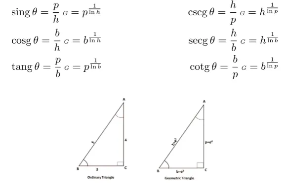
2.5. Geometric Trigonometric Ratios. Let θ be an acute angle of a geometric right
triangle and length of the sides beh, p, b∈R(G) with usual meaning. Then we define
singθ= p
hG=p 1
lnh cscgθ= h
pG =h 1 lnp
cosgθ= b
hG=b 1
lnh secgθ= h
b G =h 1 lnb
tangθ= p
bG =p 1
lnb cotgθ= b
pG=b 1 lnp
Figure 2. Geometric Right Triangle
2.6. Relation between geometric and ordinary trigonometry. Since nunit length
in ordinary coordinate system is equal to en unit in geometric coordinate system. So
properties of the geometric right triangle having sides h, p, b ∈R(G) will be same to the ordinary right triangle having sidesh0 = ln(h), p0 = ln(p) and b0 = ln(b),respectively. An example is given in FIGURE 2. Here, area of the both the triangles = 6 square unit,
∠A= 36.87◦,∠B = 53.13◦ and ∠C = 90◦.
2.7. Geometric Trigonometric Identities. We can verify that
singAcscgA=e, sing2GA⊕cosg2GA=e
cosAsecA=e, tang2GA⊕e= secg2GA
tangAcotgA=e, cotg2GA⊕e= cscg2GA.
sing(A+B) = singAcosgB⊕cosgAsingB.
cosg(A+B) = cosgAcosgB singAsingB.
2.8. G-Limit. According to Grossman and Katz [12], geometric limit of a positive valued function defined in a positive interval is same to the ordinary limit. Here, we defineG-limit of a function with the help of geometric arithmetic as follows:
A function f, which is positive in a given positive interval, is said to tend to the limit
l > 0 as x tends to a ∈ R, if, corresponding to any arbitrarily chosen number > 1, however small(but greater than 1), there exists a positive numberδ >1,such that
1<|f(x) l|G
<
for all values ofx for which 1<|x a|G
< δ.We write Glim
x→af(x) =l orf(x)
G
−→l.Here,
|x a|G
< δ⇒ a
δ < x < aδ and |f(x) l|
G
< ⇒ l
< f(x)< l.
A function f is said to tend to limit l asx tends to a from the left, if for each > 1 (however small), there existsδ >1 such that|f(x) l|G < whena/δ < x < a.In symbols
Glim
x→a−f(x) =lorf(a
−1) =l.
Similarly, a functionf is said to tend to limit lasx tends to afrom the right, if for each
>1,there existsδ >1 such that|f(x) l|G < whena < x < aδ. In symbols
Glim
x→a+f(x) =lorf(a+ 1) =l.
2.9. G-Continuity. A functionf is said to beG-continuous atx=a if (i) f(a) i.e., the value of f(x) at x=a, is a definite number,
(ii) theG-limit of the function f(x) as x−→G aexists and is equal to f(a).
Alternatively, a function f is said to be G-continuous at x = a, if for arbitrarily chosen
> 1, however small, there exists a number δ > 1 such that |f(x) f(a)|G
< for all values ofx for which,|x a|G
< δ.
It is seen that a function f isG-continuous atx=a if limx→aff(x)(a) = 1.
3. Basic Properties ofG-Calculus
3.1. G-Derivative and its Interpretation. In [5] we defined the G-differentiation of
f(x) as
dGf
dxG =f
G(x) =
Glim h→1
f(x⊕h) f(x)
h G = limh→1
f(hx)
f(x)
ln1h
for h∈R(G). (2)
TheG-derivative of a positive valued functionfat a pointcbelonging to a positive interval can be defined as
fG(c) =
Glim x→c
f(x) f(c)
x c G = limx→c
f(x)
f(c)
1 ln(xc)
Equation (3) is the bigeometric slope defined by Grossman in [13]. Depending on Grossman [13], Grossman and Katz [14], different researchers have been developing the bigeometric calculus taking arithmetic increment to the independent variable. But we are trying to develop their work with the help of geometric increments. So, to remove the confusion
among the readers, instead of the phase “bigeometric calculus” the term “G-calculus” is
used throughout the paper.
From (3), it is clear that G-derivative exists if bothf(x) and f(c) takes same sign and
at the same timex and ctakes same sign.
x+his arithmetic change andx⊕h=xhis geometric change to the independent variable
x.Now, asxchanges toxh, value of the function changes fromf(x) tof(x⊕h) =f(xh).
Geometric changes tox and y are given by
∆x=x⊕h x= xh
x =h and ∆y=f(x⊕h) f(x) =
f(xh)
f(x) .
In case of ordinary derivative ∆y∆x = f(x+h)−f(x)h gives the average additive change in f(x) per unit change inx over the interval [x, x+ ∆x] = [x, x+h].Here inG-calculus,
∆y
∆xG= (∆y) 1 ln(∆x) =
f(xh)
f(x)
ln1h
gives the average geometric change inf(x) per unit geometric change inxover the interval [x, xh].Now taking the limit as ∆x(i.e. h) tends to 1,we get
dGy
dGx = Glim
∆x→1
∆y
∆xG = G∆x→1lim
(∆y)ln(∆1x) = lim h→1
f(xh)
f(x)
ln1h .
It is to be noted that G-derivative exists iff(x)6= 0 and f(x), f(hx) are both positive or both negative.
y = mx ⊕c i.e. y = c.xlnm represents a straight line with slope m in geometric
co-ordinate system as well as in log-log paper. Then, yG = m. i.e. G-derivative is the
slope of the geometric straight line.
Note: We’ll denotenth geometric derivative byf[n].We call that left handG-derivative and right handG-derivative exist atx=c if
lim
x→c−
f(c.h)
f(c)
ln(1x c)
and lim
x→c+
f(c.h)
f(c)
ln(1x c)
exist, respectively.
Theorem 3.1. If a function f is G-differentiable and is positive, then it is both G -continuous and ordinary -continuous.
Proposition 3.1. A continuous function f is not necessarily G-derivable.
Proof. Let us consider the function
f(x) =|x|G
=
x, ifx >1
1, ifx= 1
1
x, if 0< x <1.
Then, obviously it is continuous at x = 1. But it is not G-differentiable at x = 1 as
LfG(1) =ebutRfG(1) = 1
e.
Remark 3.1. f(x) =xn is a polynomial of degree nin ordinary sense, but geometrically it is a polynomial of degree one as xn=enx.So, its G-derivative is constant.
3.2. Relation between G-derivative and ordinary derivative. By definition, G -derivative of a positive valued functionf(x) is given by
fG(x) =
Glim h→1
f(x⊕h) f(x)
h G
= lim
h→1
f(hx)
f(x)
ln1h
, which is in 1∞ indeterminate form.
Using logarithm, to transform it to 00 indeterminate form and then applying L’ Hospital
rule, we can make a relation betweenG-derivative and ordinary derivative as follows:
fG(x) = lim
h→1e ln
h
f(hx)
f(x) i 1
lnh = lim
h→1e
lnf(hx)−lnf(x)
lnh =elimh→1 hxf0(hx)
f(hx) =e
xf0(x)
f(x) . (4)
3.3. G-derivatives of some standard functions.
• G-derivative of a constant: Iff(x) =c,thenfG(x) = 1
• G-derivative of ordinary product of a constant and a function:
dG
dxG (cf(x)) =e
xcfcf0((xx))
=ex
f0(x)
f(x) = d
G
dxG (f(x)).
• G-derivative of ordinary product of two functions:
dG
dxG (f(x).g(x)) =
dG
dxG (f(x)).
dG
dxG (g(x)). (5)
• G-derivative of quotient of two functions:
dG
dxG
f(x)
g(x)
=
dG
dxG (f(x))
dG
dxG (g(x))
. (6)
• G-derivative of trigonometric functions:
dG
dxG(sinx) =e
xcotx, dG
dxG(cotx) =e
−xsecxcscx dG
dxG(cosx) =e
−xtanx, d
G
dxG(secx) =e
xtanx dG
dxG(tanx) =e
xsecxcscx, dG
dxG(cscx) =e
−xcotx.
Theorem 3.2. If f : (a, b) :−→R(G) isG-differentiable, then
(i) f is increasing, iffG ≥1.
(ii) f is decreasing, iffG ≤1.
Proof. Let c be an interior point of the domain [a, b] of a function f and fG(c) exists
and be positive, i.e. fG(c) > 1. Then, fG(c) is the limit of hf(x)
f(c) iln(x/c1 )
. Then for given
>1,∃δ >1 such that
fG(c)
<
f(x)
f(c)
ln(x/c1 )
< .fG
(c) wherex∈]c/δ, cδ[.
If >1 is so chosen that < fG(c),thenhf(x)
f(c) iln(x/c1 )
(ii) f(x)f(c) <1,i.e. f(x)< f(c) if x∈]c/δ, c[.
Thus from (i) and (ii) f(x) is increasing at x = c. Hence the function is increasing at
x=c iffG(c)>1. Similarly, it can be proved that the function is decreasing at x=c if
fG(c)<1.
Theorem 3.3(Geometric Darboux’s Theorem). If a functionf isG-derivable on a closed interval [a, b] and fG(a), fG(b) are of opposite signs (i.e. one is >1, other is <1) then
there exists at least one pointc between a andb such that fG(c) = 0.
Proof. Let fG(a) < 1 and fG(b) > 1. Since, G-derivative exists ⇒ ordinary derivative
exists, so,f0(a) and f0(b) exist. Now
fG
(a)<1⇒f0(a)<0 andfG
(b)>1⇒f0(b)>0.
From Newtonian calculus, there existsc∈[a, b] s.t. f0(c) = 0.So fG(c) =ecf 0
(c)
f(c) = 1.
Theorem 3.4(Geometric Intermediate value theorem for derivatives). If a function f is G-derivable on a closed interval [a, b]and fG(a)6=fG(b) andk be a number lying between
fG(a) and fG(b),then ∃ at least one point c∈]a, b[such that fG(c) =k.
Proof. Let g(x) = fxln(x)k.Then g
G(a) = fG(a)
k and g
G(b) = fG(b)
k .Since f
G(a)< k < fG(b),
so fGk(a) and fGk(b) can not be greater than 1 at the same time. Therefore, if gG(a) >1
then gG(b) < 1. Hence, g(x) satisfies the conditions of Darboux’s theorem. Thus, there
exists at least one pointc∈]a, b[ such thatgG(c) = 1, i.e.fG(c) =k.
Theorem 3.5 (Geometric Rolle’s Theorem). If a function f defined on[a, b]is
(i) G-continuous on [a, b],
(ii) G-derivable on ]a, b[,
(iii) f(a) =f(b),
then there exists at least one number c betweena and b such thatfG(c) = 1.
Proof. Since G-continuous functions are ordinary continuous and f0(x) exists if fG(x)
exists. So, f satisfies the conditions of G ordinary Rulle’s theorem. So, there exists
c∈]a, b[ such thatf0(c) = 0.HencefG(c) =e
cf0(c)
f(c) = 1.
Theorem 3.6 (Lagrange’s Mean Value Theorem). If a functionf defined on [a, b]is
(i) G-continuous on [a, b],
(ii) G-derivable on ]a, b[,
then there exists at least onec∈]a, b[ such that
fG
(c) =
f(b)
f(a)
1 ln(ab)
Proof. Let us define a function
φ(x) =xlnk.f(x) where the constantk is so determined thatφ(a) =φ(b).
φ(a) =φ(b)⇒alnk.f(a) =blnk.f(b)⇒ha
b ilnk
= f(b)
f(a).
Using natural logarithm to both sides we get
k=
f(b)
f(a)
1 ln(ab)
=
f(b)
f(a)
−1 ln(ab)
Now,φ(x),the product of twoG-derivable and G-continuous functions, is itself (i) G-continuous on [a, b],
(ii) G-derivable on ]a, b[,and (iii) φ(a) =φ(b).
Therefore by Geometric Rolle’s theorem∃c∈]a, b[ such thatφG(c) = 1.But
φG
(x) = d
G
dxG(x
lnk). dG
dxG(f(x)) =k.f G
(x).
⇒1 =φG(c) =k.fG(c)⇒fG(c) = 1
k =
f(b)
f(a)
1 ln(ba)
.
Note: If we replace b by ah, where h > 1, then c ∈]a, b[ may be taken as a.hlnθ for 1< θ < e. Thus
fG
(a.hlnθ) =
f(ah)
f(a)
1 ln(aha)
⇒ f(ah) =f(a). h
fG
(a.hlnθ)ilnh, where 1< θ < e.
Now we deduce geometric Taylor’s expansion forf(ah) with the help of Geometric Rolle’s
Theorem. Firstly, we have to findG-derivative of two important functions as follows.
Lemma 3.1. If y=f[n](x)
lnn(ahx)
n! then yG = [f
[n+1](x)] lnn(ahx )
n!
[f[n](x)]
ln(n−1)(ahx) (n−1)!
Proof. Taking logarithm to both sides of y and differentiating, we get
⇒ y
0 y =
d dx f
[n](x) f[n](x) .
lnn(ahx )
n! + lnf
[n](x).ln
n−1)(ah x)
(n−1)! .
−ah x2 ah x
⇒exy
0
y =ex f0[n](x)
f[n](x). lnn(ahx )
n! .exlnf[n](x).
ln(n−1)(ahx) (n−1)! .
−1
x
⇒yG
=hf[n+1](x)i
lnn(ahx)
n!
.hf[n](x)
i−ln(n
−1)(ah x )
(n−1)!
=
f[n+1](x)
lnn(ahx)
n!
f[n](x)
ln(n−1)(ahx) (n−1)!
.
Lemma 3.2. If y = klnp(ahx) where k is a constant and p is a positive integer, then
yG =k−pln(p−1)(ahx).
Proof. Taking logarithm on the both sides, and then differentiating we get the result.
Theorem 3.7 (Geometric Taylor’s Theorem). A function f defined on[a, ah]is such that
(i) the (n−1)th G-derivative of f, i.e. f[n−1] is G-continuous on[a, ah], and
(ii) the nth G-derivative, f[n] exists on [a, ah]
then there exists at least one number θ between1 ande such that
f(ah) =f(a). h
f[1](a)ilnh. h
f[2](a)
iln22!h .
h f[3](a)
iln33!h ...
...hf[n−1](a)i
lnn−1h
(n−1)!
.hf[n](a.hlnθ)i
(1−lnθ)(n−p) lnn h (n−1)!p
Proof. Condition (i) in the statement implies that f[1], f[2], f[3], ..., f[n−1] exists and are continuous on [a, ah].Let us consider the function
φ(x) = f(x). h
f[1](x)iln( ah
x )
. h
f[2](x)
i ln2(ahx)
2! ....
h
f[n−1](x)
i
lnn−1(ahx) (n−1)!
.Alnp(ahx) (8) whereA is a constant to be determined such thatφ(ah) =φ(a).
But, puttingx=ahand x=a in (8), respectively, we get
φ(ah) =f(ah), and
φ(a) =f(a). h
f[1](a)ilnh. h
f[2](a)
iln22!h ...
h
f[n−1](a)
iln
n−1h (n−1)!
.Alnph.
∴f(ah) =f(a).hf[1](a)ilnh.hf[2](a)i
ln2h
2!
...hf[n−1](a)i
lnn−1h
(n−1)!
.Alnph. (9) Now
(i) f, f[1], f[2], f[3], ..., f[n−1] all being continuous on [a, ah], the function φ(x) is con-tinuous on [a, ah];
(ii) the functions f, f[1], f[2], f[3], ..., f[n−1] and lnr(ahx ) for all r being derivable in ]a, ah[,the functionφ(x) is derivable in ]a, ah[;
(iii) φ(ah) =φ(a).
Hence,φ(x) satisfies all the conditions of Rolle’s Theorem and hence there exists one real numberθ∈]1, e[ such that φG(a.hlnθ) = 1.
Now, using Lemma 3.1 and Lemma 3.2
φG
(x) = f[1](x).
f[2](x)ln( ah
x)
f[1](x) .
f[3](x)
ln2(ahx) 2!
f[2](x)ln(ahx)
....
f[n](x)
ln(n−1)(ahx) (n−1)!
f[n−1](x)
ln(n−2)(ahx) (n−2)!
.A−pln(p−1)(ahx)
which gives
A=
h
f[n](a.hlnθ)
i(1−lnθ)(
n−p) ln(n−p)h (n−1)!p
.
Now substituting the value ofA in (9), we get
f(ah) =f(a).hf[1](a)ilnh...hf[n−1](a)i
lnn−1h
(n−1)!
.hf[n](a.hlnθ)i
(1−lnθ)(n−p) lnn h (n−1)!p
. (10)
3.4. Geometric Taylor’s Series. In (10), the term Rn = f[n](a.hlnθ)
(1−lnθ)(n−p) lnn h (n−1)!p is called Taylor’s remainder after n terms. Since, 0 < 1−lnθ < 1 as 1 < θ < e, so, (1−lnθ)n−p →0 asn→ ∞.Therefore, iff possessesG-derivative of every order in [a, ah]
thenRn→1 as n→ ∞.Then Taylor’s expansion becomes
f(ah) =f(a). h
f[1](a)ilnh... h
f[n](a)
ilnnn h!
...= Π∞n=0
h f[n](a)
ilnnn h!
. (11)
This expression can be written in terms of geometric operations as
f(a⊕h) =f(a)⊕hf[1](a)⊕ h
2G
2!G
Gf[2](a)⊕...=
∞ G
X
n=0 hnG
n!G
wherehnG =hln(n−1)h.The equivalent expressions (11) and (12) will be called respectively
as Taylor’s product and Geometric Taylor’s series.
If x ∈ [a, ah] then it also satisfies the conditions in the interval [a, x]. Then replacing
ahby x orh byx/a in (11), we get another form of Taylor’s product as follows:
f(x) =f(a). h
f[1](a)iln( x a)
. h
f[2](a)
i ln2(xa)
2! ...
h f[n](a)
i lnn(xa)
n!
...= Π∞n=0
h f[n](a)
i lnn(xa)
n! .
(13)
4. Some applications of G-calculus
4.1. Expansion of some useful functions in Taylor’s product. (i). With the help of geometric Taylor’s series, we can express different functions as a product. For example
ex=e.elnx.eln22!x.e ln3x
3! ...=e1+lnx+ ln2x
2! + ln3x
3! +...
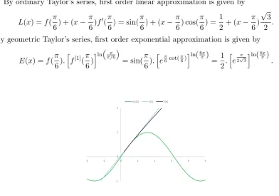
(ii). G-calculus gives better graphical and numerical approximations of functions than ordinary calculus. For, let f(x) = sin(x).In the FIGURE 3, we have given a comparison
of linear approximation and exponential approximation respectively atx= π6.
By ordinary Taylor’s series, first order linear approximation is given by
L(x) =f(π
6) + (x−
π
6)f
0
(π
6) = sin(
π
6) + (x−
π
6) cos(
π
6) = 1
2 + (x−
π
6) √
3 2 .
By geometric Taylor’s series, first order exponential approximation is given by
E(x) =f(π 6).
h f[1](π
6)
iln
x π/6
= sin(π 6).
h eπ6cot(
π
6) iln(6x
π)
= 1
2.
h e
π
2√3 iln(6x
π)
.
-1 0 1 2
-2 -1 0 1 2 3 4 5
sin(x) L(x) E(x)
Figure 3. Exponential Approximation
From the FIGURE 3, it is clear that geometric Taylor’s series gives better approximated value of the functionf(x) = sin(x) atx= π6 than Taylor’s approximation given by Michael Coco in [11] with the help of multiplicative derivative.
(iii). G-derivative gives total growth of a growth function. For, let y = a.bx, where
a=initial amount>0, b = growth(or decay) factor, x =time and y =total amount after
time periodx.Then, ddxGGy =bx,which is the total growth or total decay according tob >1
(iv). It is easy to find ordinary derivative of complicated product or quotient functions with the help ofG-derivative. For let,f(x) = e−1/x
2
xnsinx.Then
fG
(x) =
dG dxG(e
−1/x2
)
dG
dxG(xn).
dG
dxG(sinx)
= e
2/x2 en.excotx =e
2
x2−n−xcotx Therefore ordinary derivative is given by
f0(x) = f(x) ln (f
G(x))
x =
e−1/x2 xn+1sinx
2
x2 −n−xcotx
.
(v). Price Elasticity: With the aid of G-derivative, we can find price elasticity to predict
the impact of price changes on unit sales and to guide the firms profit-maximizing pricing decisions. According to [19, page no. 83], the price elasticity of demand is the ratio of the percentage change in quantity and the percentage change in the goods price, all other factors held constant. Ifxand yrepresents price and quantity respectively, then the price elasticityEp is given by
Ep = % change iny
% change inx =
∆y/y
∆x/x =x
∆y ∆x y
If price change is very small to the initially considered price, then making ∆x→0,we get
Ep =x y0
y = ln
exy
0
y
= ln(y[1]).
Resiliency =e(elasticity) =eEp =y[1]. 5. Conclusion
Bigeometric calculus is one of the most actively discussed Non-Newtonian Calculus hav-ing variety of applications. Some of such applications and advantages are discussed in our papers [4, 5]. Seeing its importance, here we discussed different properties of bigeometric calculus using geometric increments to the independent variable. We have formulated basic identities which can be expressed in terms of geometric arithmetic independently.
6. Acknowledgment
It is pleasure to thank Prof. M. Grossman and Prof. Jane Grossman for their
construc-tive suggestions and inspiring comments regarding the improvement of theG-calculus.
References
[1] A.E. Bashirov, M. Rıza, On Complex multiplicative differentiation, TWMS J. App. Eng. Math. 1(1)(2011) 75-85.
[2] A. E. Bashirov, E. Mısırlı, Y. Tandoˇgdu, A. ¨Ozyapıcı, On modeling with multiplicative differential equations, Appl. Math. J. Chinese Univ. 26(4)(2011) 425-438.
[3] A. E. Bashirov, E. M. Kurpınar, A. ¨Ozyapici, Multiplicative Calculus and its applications, J. Math. Anal. Appl. 337(2008) 36-48.
[4] Khirod Boruah and Bipan Hazarika, Application of Geometric Calculus in Numerical Analysis and Difference Sequence Spaces, arXiv:1603.09479v1, 31 May 2016.
[5] Khirod Boruah and Bipan Hazarika, Some basic properties of G-Calculus and its applications in numerical analysis, arXiv:1607.07749v1, 24 July 2016.
[7] A.F. C¸akmak and F. Ba¸sar, Certain spaces of functions over the field of non-Newtonian complex numbers, Abstr. Appl. Anal. 2014(2014), Article ID 236124, 12 pages.
[8] A.F. C¸akmak and F. Ba¸sar,On line and double integrals in the non-Newtonian sense, AIP Conference Proceedings, 1611(2014) 415-423.
[9] A.F. C¸akmak and F. Ba¸sar,Some sequence spaces and matrix transformations in multiplicative sense, TWMS J. Pure Appl. Math. 6(1)(2015) 27-37.
[10] Duff Campbell,Multiplicative Calculus and Student Projects, Department of Mathematical Sciences, United States Military Academy, West Point, NY,10996, USA.
[11] Michael Coco,Multiplicative Calculus, Lynchburg College.
[12] M. Grossman, R. Katz,Non-Newtonian Calculus, Lee Press, Piegon Cove, Massachusetts, 1972. [13] M. Grossman,Bigeometric Calculus: A System with a scale-Free Derivative, Archimedes Foundation,
Massachusetts, 1983.
[14] M. Grossman, An Introduction to non-Newtonian calculus, Int. J. Math. Educ. Sci. Technol. 10(4)(1979) 525-528.
[15] Jane Grossman, M. Grossman, R. Katz, The First Systems of Weighted Differential and Integral Calculus, University of Michigan, 1981.
[16] Jane Grossman,Meta-Calculus: Differential and Integral, University of Michigan, 1981.
[17] U. Kadak and Muharrem ¨Ozl¨uk, Generalized Runge-Kutta method with respect to non-Newtonian calculus, Abst. Appl. Anal., 2015 (2015), Article ID 594685, 10 pages.
[18] M. Riza and H. Akt¨ore,The Runge-Kutta Method in Geometric multiplicative Calculus. LMS J. Com-put. Math. 18(1)(2015) 539 - 554.
[19] W.F. Samuelson, S.G. Mark,Managerial Economics, Seventh Edition, 2012. [20] D. Stanley,A multiplicative calculus, Primus IX 4 (1999) 310-326.
[21] S. Tekin, F. Ba¸sar,Certain Sequence spaces over the non-Newtonian complex field, Abstr. Appl. Anal. 2013(2013). Article ID 739319, 11 pages.
[22] Cengiz T¨urkmen and F. Ba¸sar,Some Basic Results on the sets of Sequences with Geometric Calculus, Commun. Fac. Fci. Univ. Ank. Series A1. 61(2)(2012) 17-34.
[23] A. Uzer, Multiplicative type Complex Calculus as an alternative to the classical calculus, Comput. Math. Appl. 60(2010) 2725-2737.
Khirod Boruah is working as Research Scholar under the supervision of Bipan Hazarika at Rajiv Gandhi University, Arunachal Pradesh, India and he is study-ing on Sequence Spaces over non-Newtonian Calculus and Numerical Methods over Bigeometric Calculus.