Chain hexagonal cacti: extremal with respect to the eccentric connectivity index

Chain Hexagonal Cacti: Extremal With Respect To

The Eccentric Connectivity Index

ZAHRA YARAHMADI1,TOMISLAV DOŠLIĆ2,*AND SIROUS MORADI3

1

Department of Mathematics, Faculty of Science, Khorramabad Branch, Islamic Azad University, Khorramabad, Iran

2

Faculty of Civil Engineering, University of Zagreb, Zagreb, Croatia 3

Department of Mathematics, Faculty of Science, Arak University, Arak , Iran

(Received March 1, 2013; Accepted March 20, 2013

A

BSTRACT

In this paper we present explicit formulas for the eccentric connectivity index of three classes of chain hexagonal cacti. Further, it is shown that the extremal chain hexagonal cacti with respect to the eccentric connectivity index belong to one of the considered types. Some open problems and possible directions of further research are mentioned in the concluding section. Keywords: Chain hexagonal cactus, eccentric connectivity index.

1.

I

NTRODUCTION

The eccentric connectivity index is a graph invariant that attracted a lot of attention of researchers working in the area of QSAR/QSPR. It has been found useful in modeling various physico-chemical properties of several classes of chemical compounds [12, 20, 22]. After some initial delay, it also became a subject of a number of mathematical papers [1, 4, 6, 7, 17, 24, 25]. Here we continue with investigation of its behavior on a class of graphs of some relevance in statistical mechanics, chemistry, and theory of networks.

The central objects of this note, the cactus graphs, were introduced in the scientific literature some sixty years ago under the name of Husimi trees. They appeared in papers of Husimi [16] and Riddell [19] concerned with cluster integrals in the theory of condensation

in statistical mechanics[23]. Besides statistical mechanics, where they serve as simplified models of real lattices [18, 21], the Husimi trees were also found useful in the theory of electrical and communication networks [28] and in chemistry [15, 26].

From the mathematical point of view, the Husimi trees were first studied in a series of papers by Harary, Uhlenbeck and Norman, concerned with their enumerative properties [13, 14]. Later they become known as cactus graphs, and under that name attracted some attention when it was found out that some facility allocation problems that are NP-hard for general graphs can be solved in polynomial time for the cactus graphs [2, 27]. Also, they spawned a number of generalizations, such as block-cactus graphs [3, 29].

In this paper we study certain uniform and regular classes of cactus graphs. We present explicit formulas for the eccentric connectivity index of such cacti and show that the extremal values of this quantity are achieved on two of the considered classes.

The paper is organized as follows. In Section 2 we formally introduce the classes of graphs relevant for our investigation. Section 3 is concerned with the explicit formulas for three types of chain hexagonal cacti. In Section 4 we establish the extremal values and find the extremal chains with respect to the eccentric connectivity index. The paper is concluded by indicating some possible directions for future research.

2.

D

EFINITIONS AND

P

RELIMINARY

R

ESULTS

All graphs considered in this paper will be finite, simple and connected. For a graph G, we denote the set of its vertices by V(G) and the set of its edges by E(G).For two vertices u and

v of V(G) we define their distanced(u, v) as the length of a shortest path between u and v in

G. For a given vertex u of V(G) its eccentricity(u)is the largest distance between u and

any other vertex v of G. Hence, (u)max_vV(G)d(u,v). The eccentric connectivity index

) (G

 of a graph G is defined as



 ( ) ( ) )

(G d u  u

 ,

where d(u)denotes the degree of vertex u, i. e., the number of its neighbors in G.

A cactus graph is a connected graph in which no edge lies in more than one cycle. Consequently, each block of a cactus graph is either an edge or a cycle. If all blocks of a cactus G are cycles of the same size m, the cactus is m-uniform.

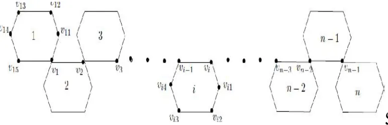
Figure 1. A Chain Hexagonal Cactus of Length 8.

Obviously, a chain hexagonal cactus of length n has 5n + 1 vertices and 6n edges. Furthermore, any chain hexagonal cactus of length greater than one has exactly two

terminal hexagons, i.e., two hexagons with only one cut-vertex. Any remaining hexagons, if present, are called internal hexagons. We denote the set of all chain hexagonal cacti of length n by (CHC)_n.It is obvious from the definition that all chain hexagonal cacti are planar, and that all their bounded faces are hexagons. A class of graphs with somewhat similar properties (planar graphs whose all bounded faces are cycles of length 6) known as

benzenoid graphs, has been studied for a long time as the mathematical model of a wide and important class of chemical compounds called benzenoid hydrocarbons. As a result, many terms of chemical origin became well established in the theory of benzenoid graphs. We adopt some of those terms and use them as a mean of concise description of three types of chain hexagonal cacti.

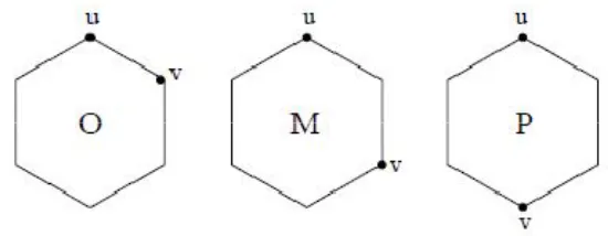
Let us consider a hexagon C6. Two vertices u and v of C6 are said to be in

ortho-position if they are neighbors in C6. If the distance between u and v is 2, they are in

meta-position. Finally, if the distance between u and v is 3, we say that they are in para-position. The ortho-, meta-, and para-position of two vertices in C6 are shown in Fig. 2.

An internal hexagon in a chain hexagonal cactus is called ortho-hexagon, meta-hexagon, or para-hexagon if its cut-vertices are in ortho-, meta-, and para-position, respectively. If all internal hexagons of a hexagonal chain cactus are of the same type, we say that the chain is regular. Obviously, three given types of internal hexagons give rise to three classes of regular chain cacti. A chain hexagonal cactus (CHC)_n is an ortho-chain if all its internal hexagons are ortho-hexagons. The meta-chain and para-chain are defined in a completely analogous manner. The ortho-chain of length n is denoted by (OC)_nand the

meta-chain is denoted by (MC)_n. The para-chain of length n will be denoted by (PC)_n. We conclude this section by noting that the number of chain hexagonal cacti grows exponentially with the number of hexagons.

Theorem 2.1. There are

 

 

 

 

      

 2

1 2

3 3 2

1 n n

different chain hexagonal cacti of length n.

The result follows by counting words of length n − 2 in a ternary alphabet and eliminating palindromes. We refer the reader to [5] for the proof.

3.

E

CCENTRIC

C

ONNECTIVITY

I

NDEX OF

R

EGULAR

C

HAINS

The unbranched nature of chain cacti allows for a natural ordering of their hexagons. It is clear that the eccentricity of vertices of a given hexagon mostly depends on the position of the hexagon in the chain and then on the way it is connected to its neighbors. The dependence is particularly simple (in fact linear) for regular chains. This fact allows us to derive explicit formulas for the eccentric connectivity index of three classes of regular chains. Throughout this section we assume n ≥ 2.

3.1. Ortho-chain.

Theorem 3.1.The eccentric connectivity index of an ortho-chain of length n is given by



(OC)_n



 

n n

n n

n n

| 2

| 2

3 36 9

36 9

2 2

 

 

 



.

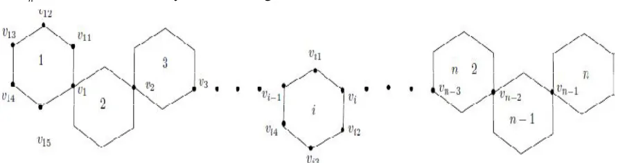
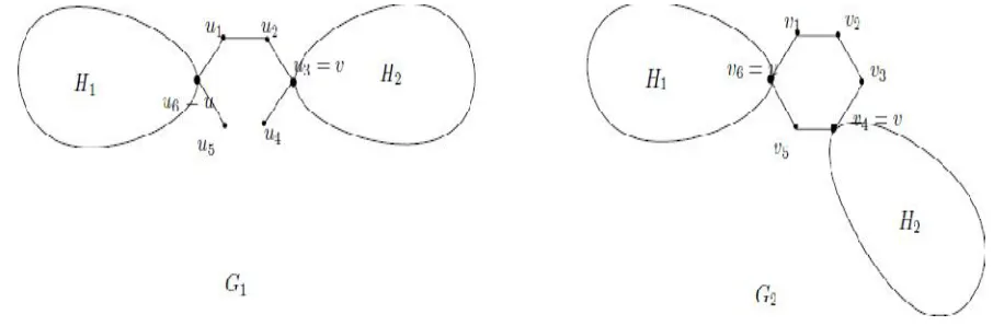
Figure 3. The Labeling of Vertices of (OC)_n.

Case 1: Let n be even, n = 2k. Because of the symmetry, it is enough to calculate the

eccentricities of vertices of first k hexagons. Their eccentricities are obtained as follows:

i. For any i,1ik,

 

v_i n2i.

ii. For any i,2ik, 

 

v_i1 n3i, 

 

v_i2 

 

v_i4 n4iand

 

v_i3 n5i.



iii. 

 

v₁₁ 

 

v₁₅ n2, 

 

v12 

 

v14 n3 and

 

v13 n4.

The total contribution of vertices of degree 2 of the i-th hexagon is now equal to



4 16 4



.

2 n  i By adding all contributions, doubling the result, and subtracting the

contribution of the middle vertex that was included twice, we obtain





_{ }

   

















. 36 9

14 5 4 4 16 4 2 2

2 4 2

4 2 ) (

2 2 /

2 2 / 1

) (

n n

n i

n

k n

i n

v v d OC

n

i n

i OC V v n

n

 

    

     









 

 



Case 2: Let n be odd, n2k1.The eccentricities of vertices in the firstk 



n1



/2 hexagons are given by the same formulas as in the even case. For the middle hexagon we have



v_k11







v_k14



n3k and 



v_k12







v_k13



n4k.The total contribution of the vertices of degree 2 in the middle hexagon is now given by



2 7 2



2



8



2 n  k  n . The other contributions remain the same as in the previous case.





_{ }

   





 













 

. 3 36 9

8 4 14 5 4 4 16 4 2 2

2 4 2

) (

2 2 / 1 2

2 / 1 1

) (

  

      

  









 

  

n n

n n

i n

i n

v v d OC

n

i n

i OC V v n

n

 

□

3.2. Meta-Chain

Theorem 3.2. Let (MC)_n be a meta-chain with n hexagons. Then the eccentric

connectivity index of (MC)_n for n > 3 is given by





.

| 2

| 2

2 18 18

18 18

)

( ₂

2

n n n

n

n n

MC _n

 

 

 

 



and



(MC)3



208.

Proof. The vertices of degree 4 and the vertices of degree 2 of first and i-th hexagons of

n

MC are labeled in the way shown in Fig. 4.

Figure 4. The Labeled Vertices of (MC)n.

Again we consider two cases.

Case1: Let n be even, n = 2k. It is enough to calculate the eccentricities of vertices of

the first k hexagons.

i. For any i,1ik,

 

v_i 2



ni



1,

ii. For any i,2ik,

 

vi1 

 

vi2 2



ni



2,

 

vi3 2



ni



3and

 

v_i4 2



ni



4.

iii. 

 

v₁₁ 

 

v₁₅ 2n,

 

v₁₂ 

 

v₁₄ 2n1and 

 

v₁₃ 2n2.

Then the total contribution of vertices of degree 2 of the i-th hexagon is equal to







8 11



.

2 ni  By the above calculation we have





_{ }

   





























. 18 18 4 10 2 . 2 11 8 2 2 1 2 4 1 2 4 2 ) ( 2 2 / 2 2 / 1 ) ( n n n i n k n i n v v d MC n i n i MC V v n n              







    

Case 2: Let n be odd, n2k1.The eccentricities of vertices of the first k hexagons

remain the same, while for the middle hexagon we have



v_k1_1



2



nk



,

 



vk12







vk14



2



nk



2

 and



v_k13



2



nk



1.Therefore





_{ }

   









 

















  . 2 18 18 9 4 2 4 10 2 2 11 8 2 2 1 2 4 2 ) ( 2 2 / 1 2 2 / 1 1 ) (               







     n n n n i n i n v v d MC n i n i MC V v n n   □ 3.3. Para-chain.

Theorem 3.3. The eccentric connectivity index of a para-chain on n vertices is given by





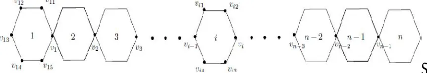
      n n n n PC _n | 2 | 2 1 27 27 ) ( ₂ 2 

Proof. We label the vertices of (PC)n in the way shown in Figure 5.

Figure 5. The Labeled Vertices of (PC)_n.

Case 1: Let n be even, n = 2k. It is enough to calculate the eccentricities of vertices of

i. For anyi, 1ik,

 

v_i 3



n1



.

ii. For any i, 2i k,

 

v_i1 

 

v_i4 3



ni



2and

 

v_i2 

 

v_i3 3



ni



1. iii. 

 

v₁₁ 

 

v₁₅ 3n2,

 

v₁₂ 

 

v₁₄ 3n1and 

 

v₁₃ 3n.

By the above calculation we have





_{ }

   





















. 27 6 15 4 6 12 2 2 12 12 2 ) ( 2 2 / 2 2 / 1 ) ( n n i n k n i n v v d PC n i n i PC V v n n           







    

Case 2: Let n be odd, n = 2k + 1. The contributions of the non-middle hexagons remain the

same, while for the middle hexagon we have



v_k11







v_k14



3



nk



and

 



v_k12





 



v_k13



3



nk



1. Therefore





_{ }

   





 





















  . 1 27 4 12 2 6 15 4 6 12 2 2 3 . 4 2 ) ( 2 2 / 1 2 2 / 1 1 ) (             







     n k n n i n i n v v d PC n i n i PC V v n n   □

As expected, all three formulas give the same value of 108 for n = 2. It is clear from the leading coefficients that for long regular chains the para-chain has the largest and the ortho-chain the smallest eccentric connectivity index. In the next section we show that those chains remain extremal also when we drop the condition of regularity.

4.

E

XTREMAL

C

HAIN

H

EXAGONAL

C

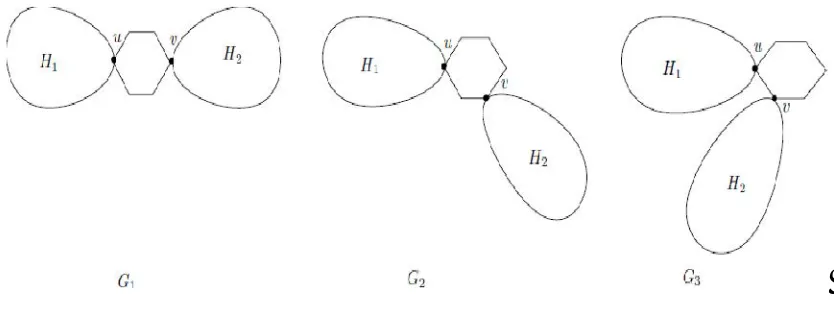
ACTI

In what follows, we prove a general theorem for obtaining extremal chain hexagonal cacti with respect to the eccentric connectivity index.

Theorem 4.1. Let H1 and H2 be connected disjoint graphs, such thatuV



H1



and



H2



V

v .The graphs G1, G2 and G3 are the graphs obtained by identifying the vertices u

and v with para-, meta- and ortho-position of vertices in C6, respectively (see Fig. 6). Then

 

G3 

 

G2 

 

G1

Figure 6. Graphs G1, G2 and G3.

Proof. There is nothing to prove if H1 or H2 is trivial, i.e., if H₁

 

u 0or  H2

 

v 0.

Hence we may assume thatd

 

u and d

 

v are at least equal to 3. It is clear that for any



H1



V



H2



V

w  its degree remains the same in all three cases, d_G1

 

w d_G2

 

w d

 

w. We start by proving the right inequality. We break the argument into 3 steps. In the first step we look at the vertices ofV



H₁



V



H₂



and compare their contributions to

 

G_{1 and}

 

G2

 .In the second step we compare the contributions of vertices u and v. Finally, in the third step, we look at the vertices of degree 2 in the hexagon C6 connecting H1 and H2.

Step 1: For any w,wV



H1





w,wV



H2





,we havedG1



w,w



dG2



w,w



. Also, for

anywV



H₁



_and wV



H₂



, we have















































,



.

, ,

,

, 2

,

, 3

,

, ,

, ,

2

2 2

2

2 2

1 2

1 1

1 1

w w d

w v d v u d u w d

w v d u

w d

w v d u

w d

w v d v u d u w d w w d

G

G G

G

G G

G G

G G

G G

 

 

 

 

 

 

 

 

 



By the above argument, we conclude that

 

 

.

2

1 w G w

G 

  for any



H1



V



H2



V

w  .In particular, we can say that if the eccentricity of



H1





w V



H2





V

w  in G1 is attained at a vertex of H1 (H2), thenG1

 

w G2

 

w . If the

eccentricity of wV



H1





wV



H2





_in G1 is attained at a vertex of H2 (H1), then

 

 

1

2 1 w  G w 

G 

 .

Step 2: Let x be a vertex of G1. We denote by

*

x _{a vertex of G1 such that}

_{ }

_

*

_

,

1 x d x x

G 



the same vertex *

x as in G1. Now we look at u and v. We claim that



2



*

H V

u  or



1



*

V H

v  .Let us suppose otherwise, i.e., *



₁



H V

u  and *



₂



H V

v  . Without loss of

generality we can assume that



*





*



, ,

1

1 u u d v v

dG  G . Then we have

 

























 

. 3

, 3

, 3

, ,

, ,

1 1 1

1 1

1 1

1

* *

* *

*

u u u d

v v d

v v d v u d v u d u u d u

G G G

G G

G G

G





 

 

 

 

 

This is a contradiction. Hence, by Step1,

 

 

 



 

1



2

1 u d u u 

u

d G G or

 

 

 



 

1



2

1 v d v v 

v

d G G . Thend

 

u G₁

 

u d

 

vG₁

 

v d

 

uG₂

 

v 3.Hence, the total contribution of u and v to

 

G₁ exceeds their total contribution to

 

G₂ .

Step 3: LetH₁

 

u mand let it be attained at vertex u*V



H1



.Similarly, letH₂

 

v land it is attained onv_*V



H₂



.Then d_H



u,u_*



m

1 and dH2



v,v*



l. Without loss of

generality we can assume m≤l. We consider two cases.

Case 1: m = l. Label the vertices of C6 in G1 and G2 as shown in Fig. 7. Then

 

₁

 

₂

 

₄

 

₅ 2

1 1

1

1 u  G u  G u  G u l

G   

 and

 

₃

 

₆ 3.

1

1 u  G u l

G 



 

₁

 

₃ 3,

 

₂ 2,

 

₅ 1

2 2

2

2 v  G v l G v l G v l

G   

 and

 

₄

 

₆ 2.

1

1 v  G v l

G 



Since the degrees of u and v in G1 and G2 are at least 3, then d

 

u d

 

v 6and by using

the eccentricity of vertices of C6 in G1 and G2, we have the following inequality:

 

 





 



 







 



 



 

 





               6 6 6 1 2 2 1 1 2 2 9 4 2 3 3 8 4 2

i G i G i

i G i G i

v v d l v d l u d l l v d l u d l u u d  

Therefore by Step 1, we conclude that 



G2





 

G1 .

Case 2: m < l. From Fig. 7 and Step 2 we obtain the following minimum values of eccentricity of vertices of degree 2 of C6 in G1 and the maximum values of eccentricity of

vertices of degree 2 of C6 in G2.

 

₁

 

₅ 2

1

1 u  G u l

G 

 and

 

₂

 

₄ 1,

1

1 u  G u l

G 



 

₁ 3,

 

₂ 2,

 

₃

 

₅ 1.

1 2

2

2 v l G v l  G v  G v l

G   

 Hence

 

 





   

   





 

 

 

 





 

 

 

 





 



























6 1 6 1

,

7

4

2

3

6

4

2

6

4

2

2 2 2 2 2 1 1 1 1

i G i G i

G

G G

i G i G i G G

v

v

v

v

d

l

v

v

d

u

u

d

l

v

v

d

u

u

d

l

u

u

d

















and by Step 1, we conclude that

 

G₂ 

 

G₁ .

By similar reasoning we can prove that

 

 

.

2

3 G

G 

  .We omit the details. Since the inequalities in Step 3 are strict, we have the following result.

Corollary 4.2. Let (CHC)n be a chain hexagonal cactus of length n. Then



(OC)_n







(CHC)_n







(PC)_n



,

   with the right (left) equality if and only if



( ) ( )



. )

( )

(CHC _n  PC _n CHC _n  OC _n

5.

C

ONCLUDING

R

EMARKS

In this section we present some results concerning the eccentric connectivity index of a family of hexagonal cacti considered in [8] and [5]. Then we show that such graphs can be also viewed as a special case of chains. That observation points toward a more general setting that encompasses in a natural way both the graphs considered here and in a series of works by Farrell [9, 10, 11].

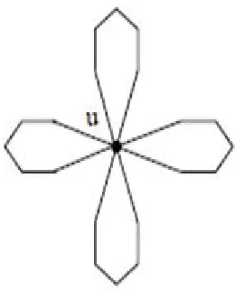
A star hexagonal cactus (SHC)n is obtained by taking n copies of C6and splicing them

Figure 8. A Star Hexagonal Cactus.

Theorem 5.1.



(SHC)_n



54n 

The star hexagonal cacti were treated separately here since the results follow by a direct computation, much easier than for the chain cacti of the previous two sections. However, star hexagonal cacti fit neatly into the class of chains by allowing the two cut vertices of all internal hexagons to coincide. Hence, a star hexagonal cactus is a “chain” hexagonal cactus whose cut-vertices are separated by a path of length 0. Now we can abandon our chemical nomenclature and index the chains by an integer parameter equal to the distance between the cut-vertices. By doing so, we obtain a uniform notation for all hexagonal cacti considered here:C_n



6,0



(SHC)_n,C_n

 

6,1 (OC)_n,C_n



6,2



(MC)_n, and

 

6,3 ( )_n.

n PC

C 

By using the above notation we can present our results by a single formula.

Theorem 5.2.













 



4



1



.

2 1 1 3

18 9

,

6 ,

2

k o n

n k kn k n k d

C        



Hered_o,k 1if k=0and 0 otherwise.

The general setting referred to at the beginning of this section now consists of considering the chain cacti Cn(m, k) made of n copies of m-gons whose cut-vertices are at

the distance k. Here we assume that . 2

   

 m

k It would be interesting to derive results for

find explicit formulas and extremal values and graphs for several generalizations of the eccentric connectivity index, such as, e.g., the augmented eccentric connectivity index.

ACKNOWLEDGMENT: Partial support of the Ministry of Science, Education and Sport of the Re-public of Croatia (Grants No. 177–0000000-0884 and 037-0000000-2779) (TD) is gratefully acknowledged.

R

EFERENCES

1. A. R. Ashrafi, T. Došlić and M. Saheli, The eccentric connectivity index of

TUC4C8(R) nanotubes, MATCH Commun. Math. Comput. Chem.65 (2011), 221–

230.

2. B. BenMoshe, B. Bhattacharya and S. Quiaosheng, Efficient algorithms for the weighted 2-center problem in a cactus graph, Lect. Notes Comput. Sci.3827 (2005), 693–703.

3. G. Chang, C. Chen and Y. Chen, Vertex and tree arboricities of graphs, J. Comb. Optim. 8 (2004), 295–306.

4. T. Došlić, A. Graovac and O. Ori, Eccentric connectivity index of hexagonal belts

and chains, MATCH Commun. Math. Comput. Chem.65 (2011), 745–752.

5. T. Došlić and F. Måløy, Chain hexagonal cacti: Matchings and independent sets,

Discrete Math.310 (2010), 1176–1190.

6. T. Došlić and M. Saheli, Eccentric connectivity index of benzenoid graphs, Novel Molecular Structure Descriptors  Theory and Applications II (I. Gutman and B. Furtula, ed.), Univ. Kragujevac, Kragujevac, 2010, pp. 169–182.

7. T. Došlić, M. Saheli and D. Vukičević, Eccentric connectivity index: extremal

graphs and values, Iranian J. Math. Chem. 1 (2) (2010), 45–56.

8. E. J. Farrell, Matchings in hexagonal cacti, Internat. J. Math. & Math. Sci. 10 (1987), 321–338.

9. E. J. Farrell, Matchings in rectangular cacti, J. Math. Sci. (Calcutta) 9 (1998), 163– 183.

10. E. J. Farrell, Matchings in pentagonal cacti, J. Math. Sci.(Calcutta) 11 (2000), 109– 126.

11. E. J. Farrell, Matchings in triangular cacti, J. Math. Sci. (Calcutta) 11 (2000), 85– 98.

13. F. Harary and R. Z. Norman, The dissimilarity characteristic of Husimi trees,

Annals Math.58 (1953), 134–141.

14. F. Harary and G. E. Uhlenbeck, On the number of Husimi trees I, Proc. Nat. Acad. Sci. USA39 (1953), 315–322.

15. H. Hosoya and K. Balasubramanian, Exact dimer statistics and characteristic polynomials of cacti lattices, Theor. Chem. Accounts76 (1989), 315–329.

16. K. Husimi, Note on Mayer’s theory of cluster integrals, J. Chem. Phys. 18 (1950), 682–684.

17. A. Ilić and I. Gutman, Eccentric connectivity index of chemical trees, MATCH Commun. Math. Comput. Chem.65 (2011), 745–752.

18. J. L. Monroe, The bilayer Ising model and a generalized Husimi tree approximation, Physica A 335 (2004), 563–576.

19. R. J. Riddell, Contributions to the theory of condensation, Ph.D. thesis, Univ. of Michigan, Ann Arbor, 1951.

20. S. Sardana and A. K. Madan, Application of graph theory: Relationship of molecular connectivity index, Wiener’sindex and eccentric connectivity index with diuretic activity, MATCH Commun. Math. Comput. Chem. 43 (2001), 85–98.

21. P. Serra, J. F. Stilck, W. L. Cavalcanti and K. D. Machado, Polymers with attractive interaction on the Husimi lattice, J. Phys. A Mat. Gen. 37 (2004), 8811–8821. 22. V. Sharma, R. Goswami and A. K. Madan, Eccentric connectivity index: A novel

highly discriminating topological descriptor for property and structure-activity studies, J. Chem. Inf. Comput. Sci.37 (1997), 273–282.

23. G. E. Uhlenbeck and G. W. Ford, Lectures in Statistical Mechanics, AMS, Providence RI, 1956.

24. Z. Yarahmadi, Eccentric connectivity and augmented eccentric connectivity in-dices of N-branched phenylacetylenes nanostar dendrimers, Iranian J. Math. Chem., 1 (2) (2010), 105110.

25. B. Zhou and Z. Du, On eccentric connectivity index, MATCH Commun. Math. Comput. Chem.63 (2010), 181–198.

26. B. Zmazek and J. Žerovnik, Computing the weighted Wiener and Szeged number on weighted cactus graphs in linear time, Croat. Chem. Acta 76 (2003), 137–143. 27. B. Zmazek and J. Žerovnik, The obnoxious center problem on weighted cactus

graphs, Discrete Appl. Math. 136 (2004), 377–386.

28. B. Zmazek and J. Žerovnik, Estimating the traffic on weighted cactus networks in linear time, Ninth International Conference on Information Visualization (IV’05), London, 2005, pp. 536–541.