Efficient elliptic curve cryptosystems

(1)

ISSN: 2008-6822 (electronic)

http://dx.doi.org/10.22075/ijnaa.2018.11642.1581

Efficient elliptic curve cryptosystems

Kamal Darweesha, Mohammad Salehb,∗

a_{Applied Mathematics Department, Palestine Technical University–Kadoorie, Tulkarm, Palestine} b_{Mathematics Department, Birzeit University, P.O. Box 14, Palestine}

(Communicated by M. Eshaghi)

Abstract

Elliptic curve cryptosystems (ECC) are new generations of public key cryptosystems that have a smaller key size for the same level of security. The exponentiation on elliptic curve is the most important operation in ECC, so when the ECC is put into practice, the major problem is how to enhance the speed of the exponentiation. It is thus of great interest to develop algorithms for exponentiation, which allow efficient implementations of ECC. In this paper, we improve efficient algorithm for exponentiation on elliptic curves defined over Fp in terms of affine coordinates. The

algorithm computes 2n2₍₂n1_P₊_Q_{) directly from random points}_P _and_Q_{on an elliptic curve, without} computing the intermediate points. Moreover, we apply the algorithm to exponentiation on elliptic curves with width–w Mutual Opposite Form (wMOF) and analyze their computational complexity. This algorithm can speed up the wMOF exponentiation of elliptic curves of size 160–bit about (21.7%) as a result of its implementation with respect to affine coordinates.

Keywords: cryptography; elliptic curves; affine coordinates.

2010 MSC: 94A60.

1. Introduction

Elliptic curve cryptosystems, which were suggested independently by Miller [7] and Koblitz [5], are new generation of public key cryptosystems that have smaller key sizes for the same level of security. The elliptic curve cryptographic operations, like encryption/ decryption schemes generation/ ver-ification signature, require computing of exponentiation on elliptic curve. The computational per-formance of elliptic curve cryptographic protocol such as Diffie–Hellman [3]. Key Exchange protocol strongly depends on the efficiency of exponentiation, because it is the costliest operation. There-fore, it is very attractive to speed up exponentiation by providing algorithms that allow efficient implementations of elliptic curve cryptosystems [1, 4, 6, 8, 9, 12].

∗_{Corresponding author}

Email addresses: [email protected] (Kamal Darweesh),[email protected](Mohammad Saleh)

(2)

There are typical methods for exponentiation such as binary methods and windowing methods [9]. These methods can speed up exponentiation by reducing additions, where addition of two points and doubling of two points are performed repeatedly.

One of the efficient windowing methods is wMOF [11]. It is a base–2 representation which provide the minimal hamming weight of exponent. Its great advantage is that it can be generated from left– to–right which means, that the recoding doesn’t have to be done in a separate stage, but can be performed on–the–fly during the evaluation. As a result, it is no longer necessary to store the whole recoded exponent, but only small parts at once.

Another approach to speed up exponentiation is by increasing the speed of doublings. One method to speed the doublings is direct computation of several doubling, which computes 2nP directly from

P ∈ E(Fq), without computing intermediate points 2P,22P, . . . ,2n−1P. Sakai and Sakurai [12]

proposed formulae for computing 2n_P _{directly (∀}_n _> _{1) on} _E₍_F

p) in terms of affine coordinates.

Since modular inversion is more expensive than multiplication, their formulae requires only one inversion for computing 2n_P _{instead of} _n _{inversions in usual add–double method.}

In this paper, we improve efficient algorithm for exponentiation on elliptic curve defined over

Fp in terms of affine coordinates. We construct efficient formulae to compute 2n2(2n1P +Q)

di-rectly from P, Q ∈ E(Fp), without computing intermediate points 2P,22P, . . . ,2n1P, 2(2n1P +

Q), . . . ,2n2−1₍₂n1_P ₊_Q_{) where} _n

1 >1. Our formulae have computational complexity (4n+ 10)M+

(4n+ 6)S+I , whereM, S and I denote multiplication, squaring and inversion respectively in Fp ,

and n=n1+n2.

Moreover, we show in which way this new algorithm for direct computing 2n2₍₂n1_P ₊_Q_{) can be} combined with wMOF exponentiation method [11]. We also implement wMOF exponentiation with and without these formulae and discuss the efficiency. The result of this implementation shows that 21.7% speed increase in wMOF exponentiation with these formulae on elliptic curve of size 160–bit. Let Fp denotes a prime finite field with p elements. We consider an elliptic curve E given

by Weierstrass non–homogeneous equation: E : y2 ₌ _x3 ₊_ax₊_b, _where _{a, b} _∈ _F

p, p > 3, and

4a3_{+ 27}_b2 _{6= 0 (i.e.} _E _{is smooth). Let}

P1 = (x1, y1), P10 = (x

0

1, y

0

1),

P2n = 2nP₁ = (x₂n, y₂n)∈E(F_p).

Let the elliptic curve point addition and doubling be denoted by ECADD and ECDBL, respectively. LetM, S and I denote multiplication, squaring and inversion, respectively in Fp, where S = 0.8M, as it is customary nowadays.

2. Previous work

In this section, we summarize the known algorithms for point addition, point doublings, and direct doublings.

2.1. Point addition

In terms of affine coordinates, point addition can be computed as follows:

Let P1 = (x1, y1), and Q= (x, y)6= O where O denotes the point at infinity, then P0 = (x0, y0) can

be computed as follows

x0 =λ2₋_x 1−x;

y0 =λ(x1−x0)−y1;

λ = (y−y1) (x−x1)

.

(3)

2.2. Point doubling

In terms of affine coordinates, point addition can be computed as follows: Assume LetP1 = (x1, y1)6=

O whereO denotes the point at infinity, then 2P =P2 = (x2, y2) can be computed as follows

x2 =λ2−2x1;

y2 =λ(x1−x2)−y1;

λ = (3x

2 1+a)

(2y1)

.

The formulae above have computational complexity 2S+ 2M +I [2].

2.3. Direct doubling

One method to increase the speed of doublings is direct computation of several doublings, which can compute 2n_P _{directly from}_P _∈_E₍_F

q), without computing the intermediate points 2P,22P, . . . ,2n−1

(see [12]).

Guajardo and Paar [4] suggested increase doubling speed by formulating algorithms for direct computation of 4P,8P, and 16P on elliptic curves over F2m in terms of affine coordinates.

Sakai and Sakurai [12] proposed formulae for computing 2nP directly (∀n _> 1) on E(Fp) in

terms of affine coordinates. These formulae require only one inversion for computing 2nP instead of

n inversions in regular add–double method.

In affine coordinate, direct computation requires only one inversion for computing 2nP instead of

n inversions in regular add–double method. Therefore direct computation of several doublings may be effective in elliptic curve exponentiation in terms of affine coordinate, since modular inversion is more expensive than modular multiplication [12].

3. Direct Computation of 2n2₍₂n1_P ₊_Q_{) in affine coordinate}

In this section, we derive formulae for computing 2n2₍₂n1_P ₊_Q_{) directly from a given points} _{P, Q}_∈ E(Fp) without computing the intermediate points 2P,22P, . . . ,2n1P,2(2n1P +Q), . . . , 2n2−1(2n1P +

Q), wheren1 ≥1, in terms of affine coordinate. These formulae can work with wMOF exponentiation

method [11].

We begin by constructing formulae for small n1, n2, then we will construct algorithm for general

n1, n2.

As an example, let n1 = 2, n2 = 1, andP1 = (x1, y1),Q= (x, y),P10(x01, y01)∈E(Fp). Then for an

elliptic curve with Weierstrass form in terms of affine coordinates P₂0 = 2P₁0 = 2(4P1+Q) = (x02, y

0

2)

can be computed as the following:

1) Computing 4P1 as in [12] 4P1 =P4 = (x4, y4) can be computed as follows:

Let

C0 =y1;

A0 =x1;

B0 = 3x21+a;

A1 =B02−8A0C02;

C1 =−8C04−B0(A1−4A0C02);

B1 = 3A21+ 16aC04;

A2 =B12−8A1C12;

(4)

Then 4P1 =P4 = (x4, y4) can be computed as follows:

x4 =

A2

(4C0C1)2

, (3.1)

y4 =

C2

(4C0C1)3

. (3.2)

2) Computing (4P1+Q)

Assume 4P1 = (x4, y4) 6= −Q, recall from Section 2, the point addition then P10 = (x

0

1, y

0

1) =

(4P1+Q) in term of affine coordinates, can be computed as follows:

x0₁ =λ2−x−x4, y10 =λ(x−x

0

1)−y. (3.3)

Substitutingx4, y4 inλ= y4

−y

x4−x we get

λ=

C2

(4C0C1)3 −y

A2

(4C0C1)2 −x

. (3.4)

Now let

T =C2−(4C0C1)3y,

S =A2−(4C0C1)2x.

Then we get:

λ = T (4C0C1)S

. (3.5)

Substituting,λ and x4 into the expression for x01, we find

x0₁ = T

2₋_S2₍_A

2+ (4C0C1)2x

(4C0C1)2S2

. (3.6)

LetM =A2+ (4C0C1)2x, we get:

x0₁ = T

2₋_{M S}2

(4C0C1)2S2

. (3.7)

LetA0₀ =T2₋_{M S}2 _{and, substituting} _λ_{, and} _x0

1 into the expression for y

0

1. Then we get:

y₁0 = −(4C0C1)

3_yS3₋_T₍_A0

0−(4C0C1)2xS2)

(4C0C1)3S3

. (3.8)

Let

C₀0 =−(4C0C1)3yS3−T(A00−(4C0C1)2xS2).

Then we get:

y₁0 = C 0

0

(4C0C1)3S3

. (3.9)

3) Computing

(5)

Recall from Section 2, the point doubling, then 2P₁0 =P₂0 = (x0₂, y₂0) in term of affine coordinates, can be computed as follows:

λ= 3A 0

0 2

+a(4C0C1)4S4

2C₀0(4C0C1)S

. (3.10)

Now, letB0₀ = 3A0₀2+a(4C0C1)4S4 and, substitutingλ, andx01 into the expression for x02. Then

we find:

x0₂ = B 0

0 2₋

8A0₀C₀02

(2C₀0)2₍₄_C

0C1)2S2

. (3.11)

LetA0₁ =B₀02−8A0₀C₀02, and substituting λ, y₁0, x0₁ and x0₂ into the expression for y0₂. Then we find

y₂0 = −8C 0

0 4₋

B₀0(A0₁−4A0₀C₀02) (2C₀0)3(4C0C1)3S3

. (3.12)

LetC₁0 =−8C₀04−B₀0(A0₁−4A0₀C₀02). Then we get finally:

y0₂ = C 0

1

(2C₀0)3(4C0C1) 3

S3. (3.13)

The formulae above have computational complexity 18S+ 22M +I.

3.1. The formulae computing 2n2₍₂n1_P ₊_Q₎ _{in affine coordinate}

From the above formulae for direct computing 2(4P1 +Q), we can easily obtain general formulae

that allow direct computing 2n2₍₂n1_P ₊_Q_{) for}_n

1 >1. Algorithm 1 describes these formulae.

Theorem 3.1 (bellow) describes the computational complexity of this formula.

Theorem 3.1. In terms of affine coordinates, there exits an algorithm that computes 2n2₍₂n1_P ₊_Q₎

at most [4(n+ 2) + 2]M, [4(n+ 1) + 2]S, and I in Fp for any point P, Q∈E(Fp) where M, S and I

denote multiplication, squaring and inversion respectively and n=n1+n2.

Proof . The complexity of step 1 and step 2 (the same as in ([12] Algorithm 1) involve (2M + 3S)n1+ (M +S)(n1−1) +S.

In step 3, we first compute

n1−1

Q

i=0

Ci which takes n1 −1 multiplication. Secondly, we perform one

squaring to compute (2n1

n1−1

Q

i=0

Ci)2. Next, we perform one multiplication to compute (2n1 n1−1

Q

i=0

Ci)2x.

Then we obtain N and V. Next, we perform two multiplications, one multiplication to compute (2n1

n1−1

Q

i=0

Ci)2y and other to compute (2n1 n1−1

Q

i=0

Ci)(2n1 n1−1

Q

i=0

Ci)2y = (2n1 n1−1

Q

i=0

Ci)3y. Then we obtain

W. Third, we perform two squaring to compute W2_, _N2_{, and one multiplication to compute} _{V N}2_.

Then we obtain A0₀. Fourth, we perform one multiplication to compute (2n1

n1−1

Q

i=0

Ci)N. Then we

obtainZ. Next, we perform two squaring to compute Z2_{, Z}4 _{and one multiplication to compute} _Z3_.

Next, we perform two multiplications to computeZ2x, Z3y. Finally, we perform one multiplication to computeW(A0₀−Z2_x_{). Then we obtain}_C0

0. The complexity of step 3 involves (n1−1)M+ 9M+ 5S.

In step 4 we perform one squaring to compute A0₀2. Next we perform one multiplication to compute

aZ4 where Z4 is computed in step 3. Then we obtain B₀0 . The complexity of step 4 involve M +S

(6)

Algorithm 1 Direct computation of 2n2₍₂n1_P ₊_Q_{) in affine coordinate, where} _n

1 > 1, and P, Q∈

E(Fp)

Input: p1 = (x1, y1), Q= (x, y)∈E(Fp)

Output: P₂0n₂ = 2n2P0 = 2n2(2n1P₁+Q) = (x0₂n2, y0₂n₂)∈E(F_p)

1. Compute A0 and C0 and B0

2. For i from 1 to n1 Compute Ai, Ci, for i from 1 to n1 -1 Compute Bi

for i= 1 ton1 do

Ai =Bi2−1−8Ai−1Ci2−1

Ci =−8Ci4−1 −Bi−1(Ai−4Ai−1Ci2−1)

end for

for i= 1 ton1−1 do Bi = 3A2i + 16ia( i−1

Q

j=0

Cj)4

3. Compute the N, V, W, Z then,

N ←An1 −(2

n1

n1−1

Q

i=0

Ci)2x

V ←An1 −(2

n1

n1−1

Q

i=0

Ci)2x

W ←Cn1−(2

n1

n1−1

Q

i=0

Ci)3y

Z ←(2k1

k1−1

Q

i=0

Ci)N

A0₀ =W2−V N2 C₀0 =−Z3_y₋_W₍_A0

0−Z2x)

4. if (n2 >0)

Compute B₀0 = 3A0₀2+aZ4

For i from 1 to n2 Compute , for i from 1 to n2 -1 Compute

for i= 1 ton2 do .Compute A0 and C0 values

A0_i =B02_i₋₁−8A0_iC02_i

C_i0 =−8C04_i₋₁−B_i0₋₁(A0_i−4A0_iC02_i)

end for

for i= 1 ton2−1 do Bi0 = 3A

02

i−1+ 16ia Z4(

i−1

Q

j=0

C0j)4 .Compute B0 values

Compute Z ←Z(2n2

n2−1

Q

i=0

C0i)

Compute x0₂n2 ←

A0n₂

Z2 , y 0

2n2 ←

Cn0₂

Z3

In step 4 we compute

n2−1

Q

i=0

C_i0 which takesn2−1 multiplications. Secondly, we perform one

multipli-cation to computeZ(2n2

n2−1

Q

i=0

C_i0). Then we obtain new value forZ. the complexity of step 4 involves

n2M. Hence, the complexity of step 4 involves 4n2M+ 4n2S.

In step 5, we perform one inversion to compute Z−1 and the result is set to T. Next, we perform one squaring to compute T2_{. Next, we perform one multiplication to compute} _A0

n2T

2_{. Then we}

obtain x0₂n₂. Finally we perform two multiplications to compute C_n0 2T

2_T_{. Then we obtain} _y0

(7)

The complexity of step 5 involves 3M +S +I. So the complexity of above computations involve [4(n+ 2) + 2]M,[4(n+ 1) + 2]S, where n=n1+n2.

3.2. Complexity comparison

For application in practice it is highly relevant to compare the complexity of 2n2₍₂n1_P ₊_Q_{) our} algorithm for direct computing of 2n2₍₂n1_P ₊_Q_{) with regular add–double method which requires} (n1+n2) separated doublings and one addition, and with Sakai–Sakuri algorithm [12] for computing

2n1+n2_P _{and 2}n2_Q_{. The performance of the new method depends on the cost factor of one inversion} relatively to the cost of one multiplication. For this purpose, we introduce, as [4], the notation of a “break even point”. It is possible to express the time that it takes to perform one inversion in terms of the equivalent number of multiplication needed per inversion.

In general let n = n1 +n2, let us denote the direct computing of 2n2(2n1P +Q) by symbol

DECDBL(n). Then our formulae can outperform the regular double and add algorithm if the fol-lowing relation to hold:

Cost(separatenECDBL+ECADD)> Cost(DECDBL(n))

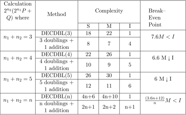
Table 1: Complexity comparison: direct computing of 2n2₍₂n1_P ₊_Q_{) vs. Individual (}_n

1+n2) doublings and one addition.

Calculation 2n2₍₂n1_P₊

Q) where Method

Complexity Break–

Even Point

S M I

n1+n2 = 3 DECDBL(3) 18 22 1 7.6M < I

3 doublings +

1 addition 8 7 4

n1+n2 = 4

DECDBL(4) 22 26 1

6.6 M ¡ I 4 doublings +

1 addition 10 9 5

n1+n2 = 5

DECDBL(5) 26 30 1

6 M ¡ I 5 doublings +

1 addition 12 11 6

n1+n2 =n DECDBL(n) 4n+6 4n+10 1 (3.6n_n+12)M < I

n doublings +

1 addition 2n+1 2n+2 n+1

Ignoring squarings and additions and expressing the Cost function in terms of multiplications and inversions, we have:

(2nM + 2nS +nI + 2M +S+I)>(4(n+ 2)M + 4(n+ 1)S+ 2M + 2S+I).

We definer =I/M (the ratio of speed between a multiplication and inversion), and assume that one squaring has complexity S = 0.8M [12]. We also assume that the cost of field addition and multiplication by small constants can be ignored. One can rewrite the above expressions as:

nrM > (2nM + 8M + 1.6nM + 4M).

Solving for r in terms ofM one obtains:

(8)

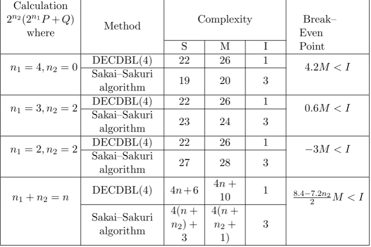
Table 2: Complexity comparison: direct computing of 2n2₍₂n1_P₊_Q_{) vs. direct computing of 2}n1+n2_P _{and 2}n2_Q_. Calculation

2n2₍₂n1_P₊_Q₎

where Method

Complexity Break–

Even Point

S M I

n1= 4, n2= 0 DECDBL(4) 22 26 1 4.2M < I

Sakai–Sakuri

algorithm 19 20 3

n1= 3, n2= 2

DECDBL(4) 22 26 1

0.6M < I

Sakai–Sakuri

algorithm 23 24 3

n1= 2, n2= 2 DECDBL(4) 22 26 1 −3M < I

Sakai–Sakuri

algorithm 27 28 3

n1+n2 =n

DECDBL(4) 4n+ 6 4n+

10 1 8.4−7.2n2

2 M < I

Sakai–Sakuri algorithm

4(n+

n2) +

3

4(n+

n2+

1)

3

As we see from Table 1, if a field inversion has complexity I > 7.6M, direct computation of 3 doublings and one addition may be more efficient than 3 separate doubling and one addition.

Moreover, our algorithm for direct computing of 2n2₍₂n1_P ₊_Q_{) can outperform Sakai–Sakuri} al-gorithm for computing 2n1+n2_P _{and 2}n2_Q_{if: Cost(direct computing of 2}n1+n2_P _{and direct computing} of 2n2_Q _{and then simply adding the two)} _> _{Cost( DECDBL(}_n

1+n2)).

In case, we ignore squaring and additions and expressing the Cost function in terms of multipli-cations and inversions, we have:

[(4n+ 1)M + (4n+ 1)S+ (4n2 + 1)M + (4n2 + 1)S+ 3I+ 2M +S]>

[4(n+ 2)M + 4(n+ 1)S+ 2M+ 2S+I].

After simplification we can rewrite the above expressions as:

2I >6M + 3S−4n2S−4n2M

Solving for r in terms ofM one obtains:

r >8.4−7.2n2

2 .

As we see from Table 2, if a field inversion has complexity I > 4.2M, direct computation of 4 doublings and one addition by using our algorithm is more efficient than 4 doublings by using Sakai– Sakuri algorithm and then performing one addition. Also, it is clear from the table and the above discussion that DECDBL(n) is different from the Sakai–Sakuri algorithm for computing 2n1+n2_P _and 2n2_Q.₂n2₍₂n1_P ₊_Q_).

3.3. Exponentiation with direct computation of 2n2₍₂n1_P ₊_Q₎

By using our previous formulae for direct computation of 2n2₍₂n1_P ₊_Q_{), where} _n

1 >1, and P, Q∈

(9)

the step 3.2 of algorithm B.1 [11] with a new step that compute 2n2₍₂n1_P ₊_Q_{) directly as in the} following algorithm.

Algorithm 2Exponentiation with wMOF Using Direct Computation of 2n2₍₂n1_P ₊_Q₎

Input: a non–zero t–bit binary string k, P ∈ E(Fp), and the multiple of the point P, γ0···tw and

ξ0···tw, the precomputed table look–up . Output: exponentiation kP.

i←t ; Q←O

while i_>0 do

if (ki XOR ki−1) = 0 then

Q←ECDBL(Q)

i←i−1

else

index←((k >>(i−w))&(2w+1₋₁₎₎₋₂w−1

if i < w then

Q←2i−(w−ξindex)+1₍₂(w−ξindex_Q₊_γ

indexP) else

Q←2ξindex₍₂(w−ξindex_Q₊_γ

indexP)

i←i−1

end if else end if else end While if i= 0 then

Q←ECDBL(Q)

if k0 = 1 then Q←ECADD(Q,−P)

return Q

In algorithm 2, for each window width w of wMOF, Step 3.1 performs direct computation of 2i−(w−ξindex)+1₍₂(w−ξindex_Q₊_γ

indexP) if (i < w) otherwise Step 3.2 performs direct computations of

2ξindex₍₂(w−ξindex_Q₊_γ

indexP) if (i>w), whereξindex= 0,1, . . . , w−1,γindexP ={±1,±3, . . . ,±(2w−1−

1)}.

3.4. Complexity analysis of the wMOF method

In this subsection, we perform an analysis of wMOF method when it used in conjunction with the 2n2₍₂n1_P ₊_Q_{) formulae. In addition, we compare the complexity of wMOF method, with and} without formulae. Moreover we derive an expression that predicts the theoretical improvement of the wMOF method by using the formulae, in terms of the ratio between inversion and multiplication times. Theorem 3.2 describes the complexity of algorithm B.1 [11] for computing exponentiation with wMOF.

Theorem 3.2. In terms of affine coordinate, let P ∈ E(Fp), t–digits exponent in wMOF, then the

complexity of algorithm B.1 [11] for computing kP requires on average

(2w+ 4)t w+ 1 M +

(2w+ 3)t w+ 1 S+

(w+ 2)t w+ 1 I,

(10)

Proof . We noticed that algorithm B.1 [11] performs an ECADD operation each time the current digit is non–zero, recall from theorem 4[11] that the average non–zero density of wMOF is asymp-totically _w1₊₁ also, one ECDBL operation is performed in each iteration (wherei_>0) to double the intermediate result. Then on average, algorithm B.1 [11] for computing exponentiation with wMOF requires

t ECDBL+ t

w+ 1ECADD.

Recall that the computational costs for doubling and additions operations in affine coordinate. Then we can rewrite previous expression as:

(2M+ 2S+I)t+ t

w+ 1(2M +S+I) We can rewrite previous expression in terms ofM, S and I as:

(2w+ 4)t w+ 1 M +

(2w+ 3)t w+ 1 S+

(w+ 2)t w+ 1 I.

Theorem 3.3. In terms of affine coordinate, let P ∈E(Fp), and t–digits exponent in wMOF, then

the complexity of algorithm 1 for computing kP requires on average

4(w+ 3)t w+ 1 M +

4(w+ 2)t w+ 1 S+

2t w+ 1I,

where M, S and I denote multiplication, squaring and inversion respectively.

Proof . Recall from [11, Theorem 4] that for t–digits exponentkin its wMOF, if t→ ∞the average non–zero density of wMOF is asymptotically _w1₊₁ and wMOF of k is infinity.

Long sequence constituted from two types of blocks: 1. b1 = (0), length of this block is 1;

2. b2 = (0i ∗0w−i−1), length of this block isw and 06i6w−1.

Then the number of blockb2 equals _w1₊₁ because every blockb2 has a non–zero bit, and the number

of block b1 equals amount of 0s in wMOF – the amount of 0s in b2 which equals

w

w+1t−(w−1)( 1

w+1)t =

t w+1.

Now, step 3.1 of algorithm 1 performs _w1₊₁t blocks b1 and step 3.2 performs _w1₊₁t block b2 then

algorithm 1 for computing kP requires on average

t

w+1ECDBL+

t

w+1DECDBL(w).

Recall the computational costs for doublings and additions operations in affine coordinate. Then we can rewrite previous expression as:

n

w+ 1(2M + 2S+I+ 4(w+ 2)M + 4(w+ 1)S+ 2M + 2S+I). We can rewrite previous expression in terms ofM, S and I as:

4(w+ 3)t w+ 1 M +

4(w+ 2)t w+ 1 S+

2t w+ 1I.

(11)

Relative improvement

Let us denote the times it would take to perform exponentiation by using algorithms B.1 [11] and 1 by symbolsTRegularmethod and TF ormulamethod, respectively. According to theorems B.1[11], and Theorem

3.1, we can derive expressions for the time it would take to perform a whole exponentiation with wMOF as:

TRegular method =

(2w+ 4)t w+ 1 M +

(2w+ 3)t w+ 1 S+

(w+ 2)t

w+ 1 I, (3.14)

TF ormula method=

4(w+ 3)t w+ 1 M +

4(w+ 2)t w+ 1 S+

2t

w+ 1I. (3.15)

From equations (3.14), and (3.15), one can readily derive the relative improvement by defining

r=I/M (the ratio of speed between a multiplication and inversion) as:

Relative Improvement= TRegular method−TF ormula method

TRegular method

. (3.16)

By using (3.14) and (3.15)

Relative Improvement= wI−[(2w+ 8)M + (2w+ 5)S]

(w+ 2)I + [(2w+ 4)M + (2w+ 3)S]. (3.17)

In our implementationS ≈M and r= 12.6, let w= 4, then

Relative Improvementis= 4(r)−29

6(r) + 23, (3.18)

Relative Improvementis = 4(12.6)−29

6(12.6) + 23 ×100 = 21.7%. (3.19)

4. Implementation and results

In this section, we implement our methods and others, which have been given in previous sections to show the actual performance of exponentiation. Implementation of an ECC system has several choices. These include selection of elliptic curve domain parameters, platforms [1].

4.1. Elliptic curves domain parameters and platforms

Generating the domain parameters for elliptic curve is vary time consuming. It consists of a suitably chosen elliptic curveEdefined over a prime finite fieldFp, and a base pointG∈E(Fp). Therefore we select NIST–recommended elliptic curves domain parameters in [10]. We implement 4 elliptic curves over prime fieldsFp, the prime modulo pare of a special type (generalized Mersenne numbers) with

log₂p= 160,192,224,256. We call these curves as P160, P192, P224 or 256 respectively. The ECC is implemented on a Pentium 4 personal computer (PC) with 2.0 GHz processor and 512 MB of RAM. Programs were written in Java language for multi–precision integer operations, and are ran under Windows XP.

4.2. Timings analysis of wMOF exponentiation method

(12)

Table 3: The ratio of speed between a multiplication and inversion in prime filed Fp.

Curves

Average Timing (msec) for M

Average Timing (msec) for S

Average Timing (msec) for I

r=I/M

P160 7.0 6.9 88.0 12.6

P192 8.7 8.6 108.8 12.5

P224 10 9.8 123.1 12.3

P256 11.9 11.8 145.2 12.2

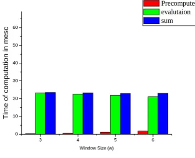
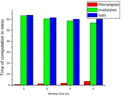
4.2.1. Optimal window size

To show the actual improvement of wMOF method with our new formula, we must find out the most efficiency proper window size, where the length of input binary form is 160–bits, 192–bits, 224– bits, or 256–bits. Figures (1– 4) illustrate the relation among the window size w, the speed of the evaluation and pre–computed processes. We can notice from these Figures that when the window size increases, time of the evaluation will decrease, while time of the precomputation will increase, and the optimal w is 4 when the input is 160–bits, and the optimal w is 5 when the inputs is 192, 224 or 256–bits. So all the tests in this paper will be processed for w = 4 in 160–bits input and

w= 5 for 192, 224, or 256–bits.

Figure 1: Pre–compute and evaluation with 160– bits input

4.2.2. The performance of improved wMOF method

Using Table 3, we can readily predict that the timings for performing a exponentiation with and without the formulae presented in Algorithm 1. In addition, using the complexity shown in equations (3.14, 3.15) and the timings shown in Table 3 we can make estimates as to how long an exponentiation with wMOF will take using both doublings with formulae and individual doublings.

5. Conclusion

In this paper, we constructed efficient algorithm for exponentiation on elliptic curve defined overFp

(13)

Table 4: Average time comparison required to perform an exponentiation without pre–computations stage of a random point in mesc (Pentium IV 2.0 GHz).

Curves Method Predicted

Timing

Measured Timing

% Improvement Predicted Measured

P 160

wMOF with

formulae (w= 4) 17.4 18.3 21.62 21.8

wMOF (w= 4) 22.2 23.4

P 192

wMOF with

formulae (w= 5 ) 23.8 24.3 25.62 25.7

wMOF (w= 5) 32 32.6

P 224

wMOF with

formulae (w= 5) 31.7 33.9 24.52 24.6

wMOF (w= 5) 42 45

P 256

wMOF with

formulae (w= 5 ) 43.8 47.4 23.5 23.3

wMOF (w= 5) 57.3 61.8

algorithm for computing 2n2₍₂n1_P ₊_Q_{) is more efficient than Sakai–Sakuri algorithm for computing} 2n1+n2_P _{and 2}n2_Q_{. A comparison was made based on notation of a “break even point”, which is the} cost factor of one inversion relatively to the cost of one multiplication. Moreover, we applied the algorithm to exponentiation on elliptic curve with wMOF and analyze its computational complexity. This algorithm can speed the wMOF exponentiation of elliptic curve of size 160–bit about (21.7%) as a result of its implementation with respect to affine coordinates.

References

[1] M. Brown, D. Hankerson, J. L´opez and A. Menezes, Software implementation of the NIST elliptic curves over prime fields, In: Naccache D. (eds) Topics in Cryptology–CT–RSA 2001. CT–RSA 2001. Lecture Notes in Com-puter Science, vol 2020. Springer, Berlin, Heidelberg.

(14)

[3] W. Diffie and M.E. Hellman, New directions in cryptography IEEE Trans. Inf. Theory, 22 (1976) 644–654. [4] J. Guajardo and Ch. Paar, Efficient algorithms for elliptic curve cryptosystems, In: Kaliski B.S. (eds) Advances

in Cryptology–CRYPTO ’97. CRYPTO 1997. Lecture Notes in Computer Science, vol 1294. Springer, Berlin, Heidelberg.

[5] N. Koblitz,Elliptic curve cryptosystems, Math. Comp., 48 (1987) 203–209.

[6] K. Koyama and Y. Tsuruoka. Speeding up elliptic cryptosystems by using a signed binary window method, In: Brickell E.F. (eds) Advances in Cryptology–CRYPTO’ 92. CRYPTO 1992. Lecture Notes in Computer Science, vol 740. Springer, Berlin, Heidelberg.

[7] V.S. Miller. Use of elliptic curves in cryptography, In: Williams H.C. (eds) Advances in Cryptology – CRYPTO ’85 Proceedings. CRYPTO 1985. Lecture Notes in Computer Science, vol 218. Springer, Berlin, Heidelberg. [8] A. Miyaji, T. Ono and H. Cohen,Efficient elliptic curve exponentiation, In: Han Y., Okamoto T., Qing S. (eds)

Information and Communications Security. ICICS 1997. Lecture Notes in Computer Science, vol 1334. Springer, Berlin, Heidelberg.

[9] B. M¨oller. Improved techniques for fast exponentiation, In: Lee P.J., Lim C.H. (eds) Information Security and Cryptology — ICISC 2002. ICISC 2002. Lecture Notes in Computer Science, vol 2587. Springer, Berlin, Heidelberg.

[10] National Institute of Standards and Technology. Digital signature standard (dss). In Pil Joong Lee and Chae Hoon Lim, editors,Information Security and Cryptology-ICISC 2002. FIPS PUB 186-2, 2000.

[11] K. Okeya, K. Schmidt–Samoa, Ch. Spahn and T. Takagi,Signed binary representations revisited, In: Franklin M. (eds) Advances in Cryptology – CRYPTO 2004. CRYPTO 2004. Lecture Notes in Computer Science, vol 3152. Springer, Berlin, Heidelberg.