Vol. 8, No. 1, 2016 Article ID IJIM-00766, 6 pages Research Article
Numerical solution of general nonlinear Fredholm-Volterra integral
equations using Chebyshev approximation
F. Fattahzadeh ∗†
Received Date: 2015-02-14 Revised Date: 2015-09-06 Accepted Date: 2015-12-22
————————————————————————————————–
Abstract
A numerical method for solving nonlinear Fredholm-Volterra integral equations of general type is presented. This method is based on replacement of unknown function by truncated series of well known Chebyshev expansion of functions. The quadrature formulas which we use to calculate integral terms have been estimated by Fast Fourier Transform (FFT). This is a grate advantage of this method which has lowest operation count in contrast to other early methods which use operational matrices (with huge number of operations) or involve intermediate numerical techniques for evaluating intermediate integrals which presented in integral equation or solve special case of nonlinear integral equations. Also rate of convergence are given. The numerical examples show the applicability and accuracy of the method.
Keywords : Nonlinear Fredholm-Volterra integral equation; Chebyshev polynomials; Error analysis; Fast Fourier Transform.
—————————————————————————————————–
1
Introduction
I
nmethodthis paper we present a computationalfor solving general nonlinear Fredholm-Volterra integral equations of the second kind:x(s) =y(s) +λ1 ∫s
0 K1(s, t)f(t, x(t)) dt+λ2
∫1
0 K2(s, t)g(t, x(t))dt,
0≤s, t≤1.
(1.1)
Several numerical methods for approximating the solution of linear and nonlinear integral equa-tions are known [1]-[19]. Brunner in [7] applied a collocation-type method and Ordokhani in [17] applied rationalized Haar function to nonlinear
∗Corresponding author. [email protected] †Department of Mathematics, Central Tehran Branch, Islamic Azad University, Tehran, Iran.
Volterra-Fredholm integral equations. A varia-tion of the Nystrom method was presented in [14]. A collocation type method was developed in [12]. Also more recent works have solved sim-ple case of these equations with operational ma-trices with more huge computations and opera-tion counts ([5],[11],[14],[15],[18],[19]). Borzabadi in [6] converted the nonlinear Fredholm integral equation to an optimal control problem and then used a linear programming to solve the problem. Orthogonal functions and polynomials receive at-tention in dealing with various problems such as integral equations. The main characteristic of us-ing orthogonal basis is that it reduces these prob-lems to solving a system of nonlinear algebraic equations by truncated approximating series
x(t)≃xN(t) = N∑−1
i=0
ciTi(t),
where function x(t) ∈ L2([0,1]) and c
n =
(f(t), Tn(t)), in which (.,.) denotes the inner
product in L2([0,1]) also C and T are matrices given by
C= [c0, c1, . . . cN]T,
T(t) = [T0(t), T1(t), . . . , TN(t)]T,
(1.2)
where Tn(t), 0 ≤ n ≤ N are Chebyshev
poly-nomials of the first kind and degree n which are orthogonal with respect to the weight function
ω(t) = 1/√1−t2 on the interval [-1,1]. These
polynomials satisfy the following recursive for-mula,
T0(t) = 1, T1(t) =t,
Tm+1(t) = 2tTm(t)−Tm−1(t), m= 1,2, . . . .
2
Fast method of solution for
general
nonlinear
integral
equations
Consider the nonlinear integral equation (1.1). At first we approximatex(t) as
x(t)≃CTT(t), (2.3)
then we substitute this approximation into eq. (1.1) to get
CTT(s) =y(s) +λ1 ∫s
0 K1(s, t) f(t,CTT(t))dt+λ
2 ∫1
0 K2(s, t) g(t,CTT(t))dt.
(2.4)
In order to use Gaussian integration formula for eq. (2.4), we transfer the intervals [0, si] and [0,1]
into interval [−1,1] by transformations
τ1 =
2
si
t−1, τ2 = 2t−1.
For Chebyshev polynomials we consider the col-location points
si = cos( iπ
N), i= 0,1, . . . , N, (2.5)
let
H1(s, t) =K1(s, t)f(t,CTT(t)), H2(s, t) =K2(s, t)g(t,CTT(t)).
Using collocation points (2.5) in transformed eq. (2.4), we get
CTT(si) =y(si)+ λ1s2i
∫1
−1H1(si,
si(τ1+1)
2 )dτ1+ λ2
2 ∫1
−1H2(si, (τ2+1)
2 )dτ2.
(2.6)
Now we use Clenshaw-Curtis quadrature formula [10] to get
CTT(si) =y(si)+ N
∑
k=0 ′′w
k[λ1 si
2H1(si,
si(sk+ 1)
2 )+
λ2
2 H2(si, (sk+1)
2 )],
(2.7)
fori= 0,1, . . . , N, where
wk =
4
N N ∑
even n=0 ′′ 1
1−n2cos( nkπ
N ), (2.8)
and double prime means that the first and the last terms are halved. The system (2.7) consist of N+1 nonlinear equations which can be solved by usual iterative method such as Newton’s method or simplex method. The Fast Fourier Transform (FFT) technique is used to evaluate the summa-tion part in (2.7) in O(NlogN) operations. In fact eq. (2.8) for weights wk can also be viewed
as the discrete cosine transformation of the vector
v with entries:
vn= {
2/(1−n2), n even
0, n odd.
The weights wk therefore is computed directly
in O(NlogN) operations, this will be the faster computation when we integrate functions in (2.6) using the same value of N. Therefore one of the good advantages of this method to all early methods which use m-power of operational ma-trices with operation cost of at least O(mN3) orO(m2N5) ([5],[9],[11],[13],[15],[18],[19]) (for the simple case (x(t))m as the nonlinear term of inte-gral equations) is that the method is reasonable in cost and also very stable against rounding er-rors as we see in the next section.
3
Convergence and error
analy-sis
Table 1: Mean absolute error for Example4.1, order of operations and CPU times.
Method of [19] N=16 e=0.0039 O(mˆ2Nˆ2) ^CP U = 4.5562
method of [5] N=16 e=1.52d-4 O(mNˆ3)
CPU=-method of [13] N=16 e=2.2011d-2 O(mˆ2Nˆ2)
CPU=-method of [12] n=8,m=8 e=2.7255 O(mˆ2Nˆ2)
CPU=-present method: N=6 e=1.21d-3 O(N lnN) CPU=4.01*10ˆ-2
N=16 e=0.66d-8 1.65*10ˆ-1
N=32 e=0.28d-15 4.13*10ˆ-1
Table 2: Absolute error of Example4.2 by introduced method (N= the number of basis functions) and their operation counts(OC).
t N=5 metod of [17] (N=16)
0.0 0.306e-3 0.0e-3
0.1 0.305e-3 0.1e-3
0.2 0.304e-3 0.0e-3
0.3 0.311e-3 0.2e-3
0.4 0.336e-3 0.1e-1
0.5 0.391e-3 0.1e-3
0.6 0.485e-3 0.1e-3
0.7 0.620e-3 0.1e-3
0.8 0.785e-3 0.0e-3
0.9 0.953e-3 0.1e-3
1.0 0.107e-3 0.1e-3
OC 8.0472 65536
Table 3: Absolute error of Example [3] by introduced method (N= the number of basis functions).
t N=3 N=5 N=7 metod of [6]
0.0 0.001e-3 0.229e-4 0.258e-5 0.2e-2
0.2 0.324e-3 0.305e-4 0.735e-5 0.1e-1
0.4 0.258e-3 0.167e-4 0.793e-5 0.2e-1
0.6 0.207e-3 0.075e-4 0.255e-5 0.1e-1
0.8 0.177e-3 0.214e-4 0.398e-5 0.0e-2
1.0 0.176e-3 0.062e-4 0.264e-5 0.1e-3
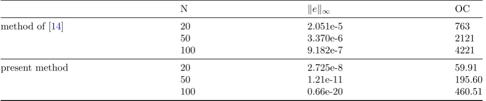
Table 4: Numerical results for Example4.4.
N ∥e∥∞ OC
method of [14] 20 2.051e-5 763
50 3.370e-6 2121
100 9.182e-7 4221
present method 20 2.725e-8 59.91
50 1.21e-11 195.60
100 0.66e-20 460.51
Proposition 3.1 Let x(t) ∈Hk(−1,1) (Sobolev
space) andTn(x(t)) = ∑n
i=0ciTi(t)be the
approx-imation polynomial ofx(t)inL2norm. Thus, the
truncation error is:
∥x(t) − Tn(x(t))∥L2[−1,1]≤ C0n−
k∥x(t)∥
on the selected norm and is independent of x(t) and n; n is the degree of Chebyshev polyno-mials (proof [8]). From proposition 3.1 it is concluded that approximation rate of Chebyshev polynomials is n−k. If x(t) is approximated by
xN(t) = ∑N
n=0cnTn(t), and we find cn ( cn is
an approximation ofcn andxN = ∑N
n=0cnTn(t))
then fort∈[−1,1], we have
∥x(t)−xN(t)∥≤C0N−k∥x(t)∥+ C2(N + 1)1/2N−k+1.
From [7] and by using closedN+ 1-point Gauss-Chebeshev rule for approximation ofcnwe realize
[11], |cn−cn|≤C1N−k+1, so it verifies the
accu-racy of the method. Given the truncated Cheby-shev series (2.3) is an approximation of eq. (1.1), it should approximately satisfy these equations, thus for each si∈[0,1],
E(si) =CTT(si)−y(si)− λ1
∫si
0 k1(si, t)f(t,C
TT(t))dt
−λ2 ∫1
0 k2(si, t)g(t,C
TT(t))dt≈0
If maxE(si) = 10−k (kis any positive integer)
is prescribed then the truncation limit N is in-creased until the difference E(si) at each points sibecomes smaller than the prescribed 10−k. We
can discuss a less strong proposition:
Proposition 3.2 Assume that (C(J),∥.∥) is the Banach space of all continuous functions on J = [0,1] with norm ∥x(s)∥= max0≤s≤1|x(s)| and the
following conditions on K1, K2 and f, g for eq.
(1.1) are satisfied and we define Ks≡K(s, t)for s, t∈[0,1],
1. lims→τ∥Ks−Kτ∥= 0, τ ∈[0,1],
2. M1 = sup0≤s,t≤1|K1(s, t)|<∞, M2 = sup0≤s,t≤1|K2(s, t)|<∞,
3. f(s, t), g(s, t) are continuous in s∈[0,1]
and Lipschitz continuous in t∈(−∞,∞), i.e. there exists a constant C1 and C2 >0 f or which
|f(s, t1)−f(s, t2)|≤C1|t1−t2|, f or all t1, t2∈(−∞,∞) and
|g(s, t1)−g(s, t2)|≤C2|t1−t2|, f or all t1, t2∈(−∞,∞),
then the solution of nonlinear equation (1.1) con-verges ([13],[16]).
Also in the L∞[0,1] we can propose as follow: Let (C[0,1],∥.∥) is the Banach space of all con-tinuous functions on interval [0,1] with∥x(t)∥∞=
maxt∈[0,1]|x(t)|. Assume |K1(s, t)|≤ M1 and
|K2(s, t)|≤ M2 and suppose the nonlinear terms f(t, x(t)) = F(t) and g(t, x(t)) = G(t) are satis-fied in Lipschitz conditions:
|F(u)−F(v)|≤L1|u−v|,
|G(u)−G(v)|≤L2|u−v|.
Moreover define α = |λ1|M1L1 +|λ2|M2L2. If x(s) and xN(s) show respectively the exact and
approximate solutions of eq. (1.1), we have
Theorem 3.1 The solution of general nonlinear Fredholm-Volterra Integral equation (1.1) by us-ing Chebyshev polynomials converges ifα ≥1; in other words limN→∞∥x(s)−xN(s)∥= 0.
Proof:
∥x(s)−xN(s)∥∞= maxs∈[0,1]
|x(s)−xN(s)|= maxs∈[0,1]|λ1 ∫s
0 K1(s, t)(F(x(t))−F(xN(t)))dt|+
maxs∈[0,1]|λ2 ∫s
0 K2(s, t)
(G(x(t))−G(xN(t)))dt|≤ |λ1|M1L1s
∥x(s)−xN(s)∥∞+|λ2|M2L2
∥x(s)−xN(s)∥∞⇒
∥x(s)−xN(s)∥∞≤α∥x(s)−xN(s)∥∞.
so the proof is completed.
4
Illustrative Examples
In this section we consider some nonlinear Fred-holm and Volterra integral equations which have been solved with other early methods such as op-erational matrix approach and solve them by in-troduced method.
Example 4.1 Consider the Fredholm integral equation
x(s) =y(s) +∫0s(s−t)x2(t)dt+ ∫1
0(s+t)x(t)dt,
(4.9)
with the exact solution x(s) =s2−2 and y(s) =
−1 30s
6+1 3s
4−s2+5 3s−
5
4. We use five methods for
this example. Table (1) shows the mean absolute error∥x−xN∥2 for equal spaced points of interval
in each methods and N stands for the number of basis functions and times are in arbitrary unit.
Example 4.2 Consider Volterra-Fredholm Hammerstein integral equation given in [12],
x(s) = 2 cos(s)−2+ 3∫0ssin(s−t)x2(t)dt+
6 7−6 cos 1
∫1
0(1−t) cos
2(s)(t+x(t))dt,
(4.10)
with the exact solution x(s) = cos(s). Table (2) shows the absolute error |x−xN|in some points
of [0,1] wherexN is the approximate solution and
N stands for the number of basis functions in the approximate solution.
Table (2) shows that by this fast method we can obtain the same results with lowest operations than do by method of [17].
Example 4.3 Consider nonlinear Fredholm in-tegral equation given in [6],
x(s) =exp(1)s+ 1− ∫ 1
0
(s+t)ex(t)dt, (4.11)
which has the exact solutionx(t) =t. As in pre-ceding examples Table (3) shows the absolute er-ror∥x−xN∥2 in some points of [0,1].
Example 4.4 Consider the following boundary value problem
x′′(t)−ex(t) = 0, 0≤t≤1,
x(0) =x(1) = 0, (4.12)
which is of grate interest in hydrodynamics [14] with exact solution
x(t) =−ln(2) + ln(λ(t)),
where
λ(t) = ( c
cos(12c(t−0.5)))
2.
Here cis the root of the equation
( c cos(4c))
2 = 2.
Problem (4.12) can be reformulated as the inte-gral equation
x(s) = ∫ 1
0
k(s, t)ex(t)dt, 0≤t≤1,
where
k(s, t) = {
−t(1−s), t≤s,
−s(1−t), s≤t.
Table 4 shows maximum error for the method of [14] and our fast method and their operation counts (OC). This table also shows that the fast method is a factor of 10 better.
5
Conclusion
As shown by numerical examples, the method in-troduced here can be simply implemented to gen-eral nonlinear integral equations of the second kind. The advantages are much less implemen-tations and fast compuimplemen-tations which is compara-ble with all huge cost early methods with simple nonlinear terms. We also have shown the conver-gence and the rate of the converconver-gence.
References
[1] K. E. Atkinson, The Numerical Solution of Integral Equations of the Second Kind, Cam-bridge University Press, 1997.
[2] E. Babolian, F. Fattahzadeh, Numerical solution of differential equations by using Chebyshev wavelet operational matrix of in-tegration, Appl. Math. Comput. 188 (2007) 417-426.
[3] E. Babolian, F. Fattahzadeh, Numeri-cal Computation method in solving integral equations by using Chebyshev wavelet oper-ational matrix of integration, Appl. Math. Comput. 188 (2007) 1016-1022.
[4] E. Babolian, A. Shahsavaran,Numerical so-lution of nonlinear Fredholm integral equa-tions of the second kind using Haar wavelets, J. Comput. Appl. Math. 225 (2009) 87-95.
[5] B. Basirat, K. Maleknejad, E. Hashem-izadeh, Operational matrix approach for the nonlinear Volterra- Fredholm integral equa-tions: Arising in physics and engineering, International Journal of the Physical Sci-ences 7 (2012) 226-233.
[6] A. K. Borzabadi, A. V. Kamyad, H. H. Mehne, A different approach for solving the nonlinear Fredholm integral equations of the second kind, Appl. Math. Comput. 173 (2006) 724-735.
[7] H. Brunner, Implicity linear collocation method for nonlinear Volterra equations, J. Appl. Numer. Math. 9 (1982) 235-247.
[9] C. Yang, Chebyshev polynomials solution of nonlinear integral equations, Journal of Franklin Institute 349 (2012) 947-956.
[10] L. M. Delves, J. L. Mohamad, Computa-tional methods for integral equations, Cam-bridge University Press, 1985.
[11] E. Hashemizadeha, K. Maleknejada, B. Basirata, Hybrid functions approach for the nonlinear Volterra-Fredholm integral equa-tions, Procedia Computer Science 3 (2011) 1189-1194.
[12] S. Kumar, I. H. Sloan, A new collocation-type method for Hammerstein integral equa-tions, J. Math. Comput. 48 (1987) 123-129.
[13] K. Maleknejad, S. Sohrabi, Y. Rostami, Nu-merical solution of nonlinear Volterra inte-gral equations of the second kind by using
Chebyshev polynomials, Appl. Math.
Com-put. 188 (2007) 123-128.
[14] K. Maleknejad, P. Torabi, Application of fixed point method for solving nonlinear Volterra-Hammerstein integral equation, U. P. B. Sci. Bull 74 (2012) 12-23.
[15] K. Maleknejad, P. Torabi, An Efficient
Computational Approach for solving a
Class of Nonlinear Integral Equations,
www.citeseerx.ist.psu.edu.
[16] K. Maleknejad, E. Hashemizadeh, B. Basirat, Computational method based on Bernstein operationa matrices for nonlin-ear Volterra-Fredholm-Hammerstein integral
equations, Commun Nonlinear Sci Numer
Simulat. 17 (2012) 52-61.
[17] Y. Ordokhani, Solution of nonlinear
Volterra-Fredholm-Hammerstein integral
equations via rationalized Haar functions, Appl. Math. Comput. 180 (2006) 436-443.
[18] Y. Ordokhani, H. Dehestani, Numerical so-lution of the nonlinear Fredholm-Volterra-Hammerstein integral equations via Bessel functions, Journal of Information and Com-puting Science 9 (2014) 123-131.
[19] A. Shahsavaran, Numerical solution of non-linear Fredholm-Volterra integral equations via picewise constant function by collocation
method, American Journal of Computational Mathematices 1 (2011) 134-138.