On Common Neighborhood Graphs II
ASMA HAMZEH1,ALI IRANMANESH1,,SAMANEH HOSSEIN−ZADEH1,MOHAMMAD ALI
HOSSEIN−ZADEH1 AND IVAN GUTMAN2
1
Department of Mathematics, Faculty of Mathematical Sciences,Tarbiat Modares University, P. O. Box 14115-137, Tehran, Iran
2
Faculty of Science, University of Kragujevac, P. O. Box 60, 34000 Kragujevac, Serbia
ARTICLE INFO ABSTRACT
Article History:
Received 3 May 2016 Accepted 12 October 2016 Published online 12 January 2018 Academic Editor: Tomislav Došlić
Let be a simple graph with vertex set ( ). The common neighborhood graph or congraph of , denoted by ( ), is a graph with vertex set ( ), in which two vertices are adjacent if and only if they have at least one common neighbor in . We compute the congraphs of some composite graphs. Using these results, the congraphs of several special graphs are determined.
© 2018 University of Kashan Press. All rights reserved Keywords:
Common neighborhood graph Congraph
Mycielski graph Shadow graph Hajós join
1
I
NTRODUCTION ANDP
RELIMINARIESLet G be a simple graph with vertex set ( ) and edge set ( ). For any vertex ∈
( ), the set of neighbors of v is the set ( ) = { ∈ ( )| ∈ ( )}. We say that
∈ ( ) is an isolated vertex if ( ) is an empty set. The distance between the vertices and of denoted by ( , ). ( ( , )for short), is defined as the length of the shortest path connecting uand v.
The complement of a graph G is a graph H on the same vertices such that two vertices of H are adjacent if and only if they are not adjacent in . The graph is usually denoted by ̅.The minimum length of a cycle in a graph Gis called the girth of G. We
Corresponding author (Email: iranmanesh@modares.ac.ir) DOI: 10.22052/ijmc.2017.53463.1195
now define several kinds of products of pairs of graphs; see [14] for details.The union of the simple graphs G and H is the graph ⋃ with vertex set ( )∪ ( ) and edge set
( )∪ ( ). If and are disjoint, then we refer to their union as a disjoint union. Suppose that and are two graphs with disjoint vertex sets. Their Cartesian product
× is a graph such that ( × ) = ( ) × ( ), and two vertices ( , ) and
( , ) are adjacent in × if and only if either = and is adjacent with , or
= and is adjacent with . The join + of the graphs G and H is the graph union ∪ together with all the edges joining ( ) and ( ). The tensor product ⨂
of the graphs and is the graph with vertex set ( ) × ( ) in which ( , ) is adjacent with ( , ) whenever ∈ ( ) and ∈ ( ). The strong product Ω
of and has the vertex set ( Ω ) = ( ) × ( ) and two distinct vertices (u1,v1)
and (u2,v2) of Ω are adjacent if = and ∈ ( )., or ∈ ( ) and
= , or ∈ ( ) and ∈ ( ).. For given vertices ∈ ( ) and ∈ ( ), a splice of and by vertices and , ( . )( , ), is defined by identifying the vertices and in the union of and [10]. Hou and Shiu [13] introduced an edge version of corona product as follows.
Let and be two graphs on disjoint sets of , vertices and , edges, respectively. The edge corona ◊ is defined as the graph obtained by taking one copy of
G and copies of , then joining two end-vertices of the i-th edge of to every vertex in the i-th copy of .
Now, we define the Hajós join which is introduced in [11]. Let and be two graphs, ∈ ( ), and ∈ ( ). Then the Hajós join of these two graphs, which is denoted by ∆ ,is a new graph that combines the two graphs by identifying vertices and into a single vertex, removing the two edges and , and adding a new edge . For example, if and are cycles of length and respectively, then the Hajós join of these two cycles is itself a cycle, of length + −1.
Let be a simple graph with vertex set { , , … , }. The common neighborhood graph (congraph) of G, denoted by ( ), is a graph with the vertex set { , , … , }.
in which two vertices are adjacent if and only if they have at least one common neighbor in the graph G [1, 2].
Congraphs have been investigated in several earlier works [1, 2, 6, 12, 15]. In [12], we obtained some results on congraphs of graph products. In this paper we continue this study and report additional results along these lines.
two. It is immediately seen that = ( ) if and only if the parent graph G does not contain triangles. Thus, in particular, = ( ) holds whenever G is bipartite.
The notations used in this paper is standard and taken mainly from [5, 14]. In what follows, the graphs considered are assumed to be simple. If a graph has parallel edges, we consider these as a single edge.
2
C
OMMONN
EIGHBORHOODG
RAPHSO
FS
OMEG
RAPHO
PERATIONSIn this section we obtain ( ) for some operations on two graphs. We begin with the tensor product. To do this, we state the following lemma which immediately follows from the definition of the operation .
Lemma 2.1. Let ( , ) and ( , ) be two vertices of ⨂ . Then ( , )∈
⨂ ( , )⋂ ⨂ ( , ) if and only if vk NG(vi)NG(vr) and
. ) ( )
(uj NH us H
N t
u
Theorem 2.2. Let G and H be two graphs without isolated vertices. Then .
) ( ) ( = )
(G H conG con H
con
Proof. Let ( , ) and ( , ) be two vertices of ⨂ such that ≠ and ≠ . If
( , )( , ) is an edge of ( ⨂ ), then there is a vertex ( , ) ∈ ( ⨂ ) such
that ( , ) ∈ ⨂ ( , )⋂ ⨂ ( , So by Lemma 2.1, ∈ ( )⋂ ( ) and
∈ ( )⋂ ( ). Therefore ∈ ( ( )) and ∈ ( ( )). This means
that for ≠ and ≠ it holds that , ( , ) is an edge of ( ⨂ ) if and
only if ∈ ( ( )) and ∈ ( ( ))..
Assume that = = . If , ( , ) is an edge of ( ⨂ ), then there is a
vertex ( , ) such that ( , )∈ ⨂ ( , )⋂ ⨂ ( , ). By Lemma 2.1, we have
∈ ( ) and ∈ ( )⋂ ( ). So if = , then ∈ ( ( )). Therefore,
for = it holds that , ( , ) is an edge of ( ⨂ ) if and only if = and
∈ ( ( )). Similarly if = , then , ( , ) is an edge of ( ⨂ ) if
and only if = and ∈ ( ( )).
Hence con(GH) = (con(G)con(H)) (con(G)con(H)) = con(G)
) (H
con and this completes the proof. ▄
Theorem 2.3. Let G and H be two graphs with the girth at least 5. Then
)) ( (
)) ( (
)) ( (
) , ))( ( ) ( ( )
(G H conG con H v x E y N x E w N v E x N y
con H G H
E(vNG(w))E((NG(v){w})(NH(x){y}))E(NG(w) y)
E(NH(y)w),
where for two vertices r, s, the notation E(r + N(s)) denotes the edges of the join of the vertex r and the neighbors of s.
Proof. In the structure of Hajós join, if we don’t remove two edges and , and don’t add a new edge , we can arrive to splice of two graphs and . So we consider the graph ( ). ( ) ( , ) as the base of the common neighborhood graph of the Hajós join of and . Then we investigate the effect of removing the two edges and , and adding a new edge .
Since the girth of the graph G is at least 5, when we remove the edge , all the edges and in ( ), ∈ ( ) and ∈ ( ), that have v and w as the common neighbor, respectively, will be deleted. Similarly when we eliminate the edge , all the edges and xb in ( ), ∈ ( ) and ∈ ( ), that have and as the common neighbor, respectively, will be deleted. Continuing this argument, when we identify the vertices and into a single vertex, then ( )− and ( )− will have a common
neighbor. So each vertex in ( )− will be adjacent to each vertex in ( )− . By adding the new edge , will become the common neighbor between and ( ) and
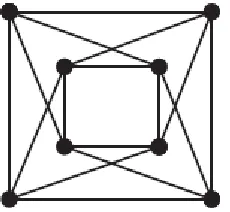
the common neighbor between and ( ). ▄ Applying the Hajós join to two copies of by identifying a vertex from each copy into a single vertex, deleting an edge incident to the combined vertex within each subgraph, and adding a new edge connecting the endpoints of the deleted edges, produces the Moser spindle, see Fig. 1. As an application we characterize the common neighborhood graph of the Moser spindle.
Figure 1. The Moser Spindle Graph.
In the next theorem, we compute the common neighborhood graph of the edge corona product of graphs. One can see that the edge corona product of with a complete graph , and the common neighborhood graph of are subgraphs of ◊ .
Theorem 2.5. Let be a graph with vertices and edges and be a graph with vertices. Then
( ) ( )
) ( ) ( ) ( = )( = G i G j k
j v i v k e
t con G N v N v H
K G H G
con
)). (
( = , = i j
q v l v j e q v l v i
e H H
Proof. Let = { , … , }, ( ) = { , … , }, and ( ) = { , … , }. Denote the i-th copy of H in ◊ , by . Each two vertices of have the end vertices of as common neighbors, So the induced subgraph of ( ◊ ) on each is a complete graph. On the other hand, a vertex in has a common neighbor with a vertex in if and only if the
edges and are adjacent. So the induced subgraph of ◊ on the vertices ⋃ is
+ if and only if and are adjacent in and there is no edge between and if and are not adjacent in .
We now consider the vertices { , … , }. Clearly, and have a common neighbor in ◊ if and only if is their common neighbor in . Also and have
a common neighbor in ◊ , if and only if is an edge of G.
Finally, a vertex in has a common neighbor with a vertex in if and only
if is in ( )⋃ , where = . This completes the proof. ▄
By definition, the edge corona ◊ of a tree of order and is the graph obtained by taking one copy of and −1 copies of and then joining two end-vertices of the i-th edge of to every vertex in the i-th copy of .
Corollary 2.6. The common neighborhood graph of the edge corona product of graphs and satisfies con(K2Sn)= Kn2 .
3.
R
ELATIONB
ETWEENS
OMES
PECIALG
RAPHSA
NDT
HEIRC
ONGRAPHSIn this section we compute the common neighborhood graphs of the central graph, line graph, shadow graph, and Mycielski graph.So we should first define these graphs.
For a given graph , the line graph of is denoted by ( ) and the vertices of
( ) are the edges of . Two edges of that share a vertex are considered to be adjacent
obtained by inserting an additional vertex in each edge of . Equivalently, each edge of is replaced by a path of length 2.
For a given graph , we do an operation on by subdividing each edge exactly once and joining each pair of vertices of the original graph which were previously non-adjacent. The graph obtained by this process is said to be the central graph of , denoted by
( ), [17, 18, 19].
The shadow graph ( ) of a connected graph is constructed by taking two
copies of say ′ and " and joining each vertex ′ in ′ to the neighbors of the corresponding vertex ʺ in ". For example, ( ) is depicted in Fig. 2.
Figure 2. The Shadow Graph D2(C4).
The Mycielski graph of G was introduced by J. Mycielski [16] for the purpose of constructing triangle–free graphs with arbitrarily large chromatic number. This graph has been much studied [7, 8, 9].
Let be a graph with vertex set { , , … , }. The Mycielski graph ( ) of contains itself as an isomorphic subgraph, together with + 1 additional vertices: a vertex which corresponds to each vertex of , and another vertex . Each vertex is connected by an edge to , so that these vertices form a subgraph in the form of a star , . In addition, for each edge of , the Mycielski graph includes two edges, and . In Fig. 3 we shows Mycielski’s construction applied to a 5-vertex cycle. The resulting Mycielskian is the Grötzsch graph, an 11-vertex graph with 20 edges. The Grötzsch graph is the smallest triangle–free 4-chromatic graph.
Theorem 3.1. Let G be a graph. Then
[ ( ( ) ( ( ) ( )))]
.) ( ) ( =
)) (
(C G G L G con G = ( ) v V G N u N v
Figure 3. The Grötzsch Graph.
Proof. Let ( ) = { , … , } and ( ) = { , … , }. So the set of vertices of ( ) is
( ) = { , … , , , … , }, where is the vertex inserted in the edge ,
)
(1im . We determine the graph ( ( )) in three steps:
(i) We find the edges between the vertices of { , … , }. The vertices and
have a common neighbor in the set { , … , }, of graph ( ) if and only if is an edge in the graph . Also the vertices and have a common neighbor in the set
{ , … , } of the graph ( ) if and only if and have a common neighbor in the graph
̅. So the subgraph induced by the vertices , … , in the graph ( ) is ⋃ ( ̅).
(ii) We consider the subgraph of C(G) induced by the set { , … , },. It is easy
to see that and do not have common neighbors in { , … , },. On the other hand,
and have the vertex as common neighbor in { , … , }. if and only if the
edges and have the vertex as the common vertex in . Therefore the respective induced subgraph is ( ).
(iii) We find the edges between {v1,v2,,vn} and { , , }
1 em
e v
v . Let ei =vrvs be an
edge of G. So ( ) = { , } and this means that is adjacent in ( ( )) to the vertices that are neighbors of and . By the definition of ( ), the edges between
{ , , … , } and { , … , } are ⋃ ∈ ( )[ + ( )− ( )⋃ ( ) ].
Combining (i), (ii), and (iii), the theorem follows. ▄
In the graph , let { , … , }be all of the edges incident to vertex . We denote the set of { , … , } in the graph ( ) by ( ). That is a vertex of ( ) corresponding
Theorem 3.2. Let G be a graph. Then con(L(G))=e=uvE(G)(NG' (u) NG' (v)).
Proof. Consider the vertices { , … , } in ( ). If = is an edge in , then
can be as the common neighbor of the sets ′ ( ) and ′ ( ). So for each = in
, ( ) + ( ) is the subgraph of ( ( )). ▄
Theorem 3.3. Let G be a graph without isolated vertices and G and G be two copies of
G. Then con(D2(G))= D2(con(G)){vi'vi"|vi'V(G),v"iV(G),1i|V(G)|}.
Proof. Suppose that ( ) = { , , … , }, ( ′) = { ′ , ′ , … , ′ }, and ( ′′) =
{ ′′ , ′′ , … , ′′ },. By definition of the shadow graph, it is easy to see that ∈
( )⋂ ( ) if and only if ∈ ( )⋂ ( ). Similarly,
∈ ( )⋂ ( ) if and only if ∈ ( )⋂ ( ). Therefore, the subgraph
of ( ( )) induced on ( ) is ( ) and induced on ( ′′) is ( ). ▄
We now determine the edges between ( ) and ( ). To do this, for two vertices and , ≠ , we use the following facts resulting from the definition of shadow graph:
1)vk' NG(vi')NG(v"j) if and only if ( ) ( )
" '
"
j G i G
k N v N v
v .
2) vk' NG(vi')NG(v'j) if and only if ( ) ( )
" '
'
j G i G
k N v N v
v .
Therefore, is an edge of ( ) if and only if ′ and ′ are edges of ( ( )). On the other hand, since G has no isolated vertices, for each i, 1≤ ≤| ( )|, are
edges of ( ( )). and the proof is completed. ▄
Corollary 3.4. For path Pn and complete graph K2 the following equality holds:
. ) ( = )) (
(D2 P con P K2
con n n
Theorem 3.5. Let be a graph with vertices. Then the congraph of its Mycielski graph contains ( ) as an isomorphic subgraph, together with + 1 additional vertices: a vertex corresponding to each vertex of ( ) such that the induced graph of ( )
on them is and another vertex . Each vertex is connected by an edge to , so that these vertices form a subgraph in the form of a star , . In addition, for each edge of
( ), the common neighborhood graph of the Mycielski graph includes two edges,
Proof. Since in the Mycielski graph, each vertex is connected by an edge to , so vertex is the common neighborhood of vertices , … , in the graph ( ) and this implies that the subgraph of ( ) induced on these vertices is . It is clear that ∈
( )( )⋂ ( )( ) if and only if ∈ ( )( )⋂ ( )( ), so the subgraph of ( )
induced on { , … , } is ( ). Also by the definition of Mycielski graph, since has not isolated vertices, the vertices are common neighborhoods of the vertices and . This implies that, 1imare edges of ( ( ) ).
Now we obtain the edges between { , … , } and { , … , }. Let the vertex be the common neighbor of the vertices and . By the definition of Mycielski graph, we have the following cases:
Case 1. The vertex is in the common neighborhood of vertices and in graph . This implies that , 1≤ ≤ are edges of the congraph.
Case 2. The vertex vk is in the common neighborhood of the vertices and , and in graph . This implies that for each edge of ( ), the common neighborhood graph of ( ) includes two edges and and this completes the proof. ▄
As an application we compute the common neighborhood graph of Grötzsch graph.
Corollary 3.6. Let C5:v1v2v3v4v5v1 . Then the common neighborhood graph of the Grötzsch
graph is determined via (wC5)K5{viui1|1i4}{vi1ui |1i4}v1u5v5u1.
R
EFERENCES1. A. Alwardi, B. Arsić, I. Gutman, N. D. Soner, The common neighborhood graph and its energy, Iranian J. Math. Sci. Inform. 7 (2012) 1–8.
2. A. Alwardi, N. D. Soner, I. Gutman, On the common–neighborhood energy of a graph,
Bull. Acad. Serbe Sci. Arts (Cl. Sci. Math. Natur.) 143 (2011) 49–59.
3. S. K. Ayyaswamy, S. Balachandran, I. Gutman, On second–stage spectrum and energy of a graph, Kragujevac J. Math. 34 (2010) 139–146.
4. S. K. Ayyaswamy, S. Balachandran, K. Kannan, Bounds on the second stage spectral radius of graphs, Int. J. Math. Sci. 1 (2009) 223–226.
5. J. A. Bondy, U. S. R. Murty, Graph Theory, Springer, New York, 2008.
6. A. S. Bonifácio, R. R. Rosa, I. Gutman, N. M. M. de Abreu, Complete common neighborhood graphs, Proc. Congreso Latino–Iberoamericano de Investigación Operativa & Simpósio Brasileiro de Pesquisa Operacional (2012) 4026–4032.
8. V. Chvátal, The minimality of the Mycielski graph, Lecture Notes Math. 406 (1974) 243–246.
9. K. L. Collins, K. Tysdal, Dependent edges in Mycielski graphs and colorings of 4-skeletons, J. Graph Theory46 (2004) 285–296.
10.T. Došlić, Splices, links, and their degree-weighted Wiener polynomials, Graph Theory Notes New York 48 (2005) 47–55.
11.G. Hajós, Über eine Konstruktion nicht n-färbbarer Graphen, Wiss. Z. Martin Luther Univ. 10 (1961) 116–117.
12.S. Hossein–Zadeh, A. Iranmanesh, A. Hamzeh, M. A. Hosseinzadeh, On the common neighborhood graphs, El. Notes Discr. Math. 45 (2014) 51–56.
13.Y. Hou, W. C. Shiu, The spectrum of the edge corona of two graphs, El. J. Lin. Algebra
20 (2010) 586–594.
14.W. Imrich, S. Klavžar, Product of Graphs – Structure and Recognition, Wiley, New York, 2000.
15.M. Knor, B. Lužar, R. Škrekovski, I. Gutman, On Wiener index of common neighborhood graphs, MATCH Commun. Math. Comput. Chem. 72 (2014) 321–332. 16.J. Mycielski, Sur le colouriage des graphes, Colloq. Math. 3 (1955) 161-162.
17.J. Vernold Vivin, Harmonious coloring of total graphs, n-leaf, central graphs and circumdetic graphs, Ph. D. Thesis, Bharathiar Univ., Coimbatore, India, 2007.
18.J. Vernold Vivin, M. M. Akbar Ali, K. Thilagavathi, Harmonious coloring on central graphs of odd cycles and complete graphs, Proc. Int. Conf. Math. Comput. Sci., Loyola College, Chennai, India, 1−3 (2007) 74–78.