VOLUME 39, ARTICLE 20, PAGES 593
,
634
PUBLISHED 25 SEPTEMBER 2018
https://www.demographic-research.org/Volumes/Vol39/20/ DOI: 10.4054/DemRes.2018.39.20
Research Article
Fewer mothers with more colleges?
The impacts of expansion in higher education on
first marriage and first childbirth
Seongsoo Choi
© 2018 Seongsoo Choi.
This open-access work is published under the terms of the Creative Commons Attribution 3.0 Germany (CC BY 3.0 DE), which permits use, reproduction, and distribution in any medium, provided the original author(s) and source are given credit.
1 Introduction 594 2 The effects of college expansion on marriage and fertility in the
transition to lowest-low fertility
596
2.1 Quantity effect 597
2.2 Return effect 598
3 The South Korean context 599
4 Data and method 601
4.1 Data 601
4.2 Analytical strategy 602
4.3 Variables 605
5 Results 607
5.1 College expansion effects on age-specific transition rates of first
marriage and first birth 607
5.2 Unobserved heterogeneity 613
6 Conclusion and discussion 616
References 621
Fewer mothers with more colleges?
The impacts of expansion in higher education on first marriage and
first childbirth
Seongsoo Choi1
Abstract
BACKGROUND
Since the mid-1990s, South Korea has undergone two remarkable social changes: a large-scale expansion in higher education and a transition to lowest-low fertility. These changes offer an appropriate quasi-experimental setting for the causal inferences of the impacts of college education on transitions into marriage and parenthood.
OBJECTIVE
I examine the effects of the large-scale college expansion on first marriage and first childbirth, using data from South Korea.
METHODS
I define two cohorts of women depending on their exposure to the expansion (pre-expansion versus post-(pre-expansion), and from this I identify a marginal group affected by the college expansion. Using a difference-in-difference approach, I examine how marriage and childbirth changes in this group (the New College Class) differed in comparison with the changes in other groups (the High School Class and the Traditional College Class).
RESULTS
I found a considerable impact of college expansion on the falling rates of first marriage and first childbirth among the New College Class women. The growing divide in family formation between college graduates and non-college graduates explains a large part of the total college expansion effects, while the effect of increased education among New College Class women was minimal.
CONCLUSIONS
The college expansion in South Korea did have an impact, but the impact was mostly indirect from interactions with other social structural changes.
CONTRIBUTION
I provide causal evidence on the impact of the large-scale expansion in higher education on family formation, in particular fertility, utilizing a novel analytical approach and a rare empirical case in South Korea.
1. Introduction
Since the instances of lowest-low fertility were first observed in Europe in the early 1990s and the term ‘lowest-low fertility’ was coined (Kohler, Billari, and Ortega 2002), researchers have explored the various factors that have led to these transitions (Billari 2005, 2008; Billari and Kohler 2004; Frejka, Jones, and Sardon 2010; Goldstein, Sobotka, and Jasilioniene 2009; Jones 2007; Kohler, Billari, and Ortega 2002; McDonald 2006). Education, particularly the increasing participation of women in postsecondary education, has been considered a major contributing factor (Billari 2005; Kohler, Billari, and Ortega 2002). For example, Italy and Spain, the leading forerunners of lowest-low fertility in the 1990s, demonstrate the most marked increases in the proportion of college-educated women in Europe (Kohler, Billari, and Ortega 2002). This suggests a plausible causal link between college expansion and fertility decline to the very low level.
Over approximately ten years, a group of East Asian countries, including South Korea, Taiwan, Japan, and Singapore, joined the lowest-low fertility club, while most European nations that had been at low levels rebound (Goldstein, Sobotka, and Jasilioniene 2009). A common feature shared by these East Asian countries is that their college education expanded sharply at the same time that their fertility fell to the lowest-low level. Given theoretical reasons and empirical evidence about substantive relationships between college education and fertility changes in these demographic transitions (Brewster and Rindfuss 2000; Kohler, Billari, and Ortega 2002; Lesthaeghe 2010; Rindfuss, Morgan, and Offutt 1996), this concurrence raises the question of whether and how large-scale college expansion influences fertility decline in the context of low fertility.
2004). In addition, most existing studies implicitly or explicitly deal with the average effect of college education, assuming that college effects on marriage and childbearing have been the same for all individuals in the population. The absence of consideration of heterogeneity is a general feature in research on fertility and higher education (Brand and Davis 2011). When college education expands because of a policy change, not all individuals respond equally to the change. Recognizing a marginal group of people who respond to the policy of college expansion by deciding to attend college is important because their experiences identify the causal effects of college expansion.
In this vein, South Korea offers a rare empirical context in which a transition from below-replacement fertility to the lowest-low level fertility occurred simultaneously with a dramatic expansion of college education during a relatively short period. As illustrated in Figure 1, college education expanded remarkably. The proportion of high school graduates who enrolled in some form of college rose from 32% in 1992 to 78% in 2003. This shift in the status of college graduates from the minority to the majority in each cohort suggests the presence of a large proportion of new college graduates who were drawn to college because of the college expansion. On the other hand, the trend of total fertility rate (TFR) suggests that, for the cohorts of people who completed high school and became eligible to attend college right before college enrollment took off in the 1990s, TFR at the prime age for entering into marriage and parenthood remained between 1.5 and 2. The equivalent rate among the post-expansion cohorts is below the lowest-low threshold at 1.3.
In this paper, I examine whether this temporal overlap results from a causal link between college expansion and marriage and fertility outcomes. I address this issue by examining the changes in entry into marriage and motherhood among women who became college graduates because of college expansion (the New College Class, NCC). This is examined relative to women whose decisions were not affected by the college expansion either because they did not attend college in either the pre-expansion or the post-expansion periods (the High School Class, HSC) or because they would attend in any case (the Traditional College Class, TCC).2 NCC is the marginal group whose members changed their college-going decision from not going to college to going to college as a response to the expanded opportunity for more education. Any changes the New College Class undergoes through the years of college expansion, therefore, present the consequences of college expansion directly or indirectly.
2 This definition of the groups with heterogeneous responses to the treatment (college expansion) assumes
Figure 1: College expansion and changes in the total fertility rate in South Korea
Source: Korean Education Statistics Service (http://cesi.kedi.re.kr/eng/index) and Korean Statistical Information Service (http://kosis.kr/eng/).
2. The effects of college expansion on marriage and fertility in the
transition to lowest-low fertility
2.1 Quantity effect
The increased quantity of education due to college expansion can contribute to changes in marriage and fertility for new college graduates. This quantity effect holds only for the New College Class as the marginal group. Existing research advances several causal mechanisms explaining how a quantitative upgrade in education affects marriage and fertility decisions.
First, a longer stay in school due to the extension of education to the postsecondary level is responsible for the postponement of marriage and parenthood (Blossfeld 1995; Blossfeld and Huinink 1991; Mills et al. 2011; Skirbekk, Kohler, and Prskawetz 2004). The roles of student and mother are difficult to balance (Mills et al. 2011), so an extension of the average length of education due to educational expansion is related to the rise of the mean age at first birth. This has been a crucial factor preceding the onset of the transition to lowest-low fertility in many countries (Goldstein, Sobotka, and Jasilioniene 2009; Kohler, Billari, and Ortega 2002). The rates of marriage and fertility are likely to decline when a substantial proportion of women, such as NCC, stay in education for longer and delay marriage. Prior research suggests that prolonged school enrollment due to educational expansion is associated with the delayed timing of marriage and motherhood and, as a consequence, a fertility decline (Blossfeld 1995; Neels et al. 2014; Neels and Wachter 2010; Ní Bhrolcháin and Beaujouan 2012). However, this association does not necessarily reflect a causal effect. For example, recent evidence from UK data demonstrates that only a very small proportion of fertility postponement, 1.9 months of the 2.74 years, is attributable to the causal effect of educational expansion (Tropf and Mandemakers 2017).
Another mechanism involved is that college education increases the human capital of women in NCC, and this enables women to access new opportunities, leading to higher socioeconomic status in the labor market compared with their HSC counterparts, and ultimately increases the opportunity costs of having a family. Higher opportunity costs create a reduced desire for children or a greater likelihood of postponing the transition to motherhood to later ages (Becker 1991; Blossfeld and Huinink 1991). Women deliberately choose the timing of first births that would yield the optimal long-term consequences with respect to their careers and wages (Gustafsson 2001; Happel, Hill, and Low 1984). As a result, a delay in first birth, again, affects the tempo of total fertility.
learn about contraceptive use in college (Cleland 2001; Goldin and Katz 2002). School-based social relationships provide social networks for the diffusion of fertility-related knowledge, attitudes, and behaviors (Cleland 2001), and these cultural and ideational changes that college education brings about can affect the timing and preference for marriage and motherhood.
2.2 Return effect
Another way college expansion affects family formation is through changing differences in marriage and childbearing between non-college-educated women and college-educated women. If the college differences in marriage or childbirth widen or narrow during the period of college expansion for reasons that are not necessarily related to college expansion, this also affects the amount of total change the New College Class experiences. The return effect holds for all college graduates, including both the New and Traditional College Classes.
These changes in the educational gradient of marriage or fertility may be induced by social and economic factors that influence women’s family formation decisions unequally across educational groups. For example, skill-biased technological changes in the labor market increase demand for college graduates, thereby resulting in a higher college premium in earnings (Goldin and Katz 2008). This raises the opportunity costs of marriage and childbearing among college-educated women. Growing economic uncertainty that stems from other macroeconomic changes, such as an economic recession, can also disproportionately increase the costs of having a child for college graduates compared with non-college graduates (Adserà 2004; Ahn and Mira 2001; Sobotka, Skirbekk, and Philipov 2011). During economic hardship, better-educated women also have difficulty finding a partner who meets their minimum level of expected economic security (Ahn and Mira 2001; Sobotka, Skirbekk, and Philipov 2011), and this can engender an education gap in marriage. The increasing availability of high quality daycare facilities is another possible source of the return effect, as college-educated women are more likely to benefit from the change (Kravdal and Rindfuss 2008).
Witsberger 1986). This may be true especially when social change triggers disagreement between existing social norms and a new reality.
The spillover or externality of college expansion in labor markets and marriage markets is also a possible source of the return effect. Those in TCC are not affected by college expansion when making educational decisions, but a large-scale inflow of NCC women may affect their relative statuses in job markets and marriage markets. For example, a rise in the supply of college graduates due to the sharp expansion in higher education lowers the college premium in wages, holding the skill demand constant, leading to a fall in economic opportunity costs of marriage and motherhood for female college graduates. In this case, a college expansion may create a negative quantity effect and a positive return effect. This is also true for HSC.
3. The South Korean context
The dramatic expansion of college education in South Korea was mainly a product of government policies. From the early 1990s, the South Korean government began to promote technical and vocational education at the secondary and postsecondary levels. This policy initiative led to a sharp increase in the number of technical and vocational schools at secondary and postsecondary levels, including junior colleges. The number of junior colleges increased sharply from 127 in 1993 to 161 in 1999. Another significant policy change that drove the expansion was the education reform in 1995. The reform simplified the procedures for establishing 4-year private universities (Choi 2015; Lee, Jeong, and Hong 2014). Within three years after the policy had taken effect, 25 new 4-year universities were established, and between 1995 and 2005, the number of students enrolling in 4-year institutions increased by 55%. The sharp expansion of college education in South Korea in the 1990s was largely induced by policy changes, and so it had an exogenous origin.
As illustrated in Figure 1, entries into marriage and parenthood also changed notably in South Korea during the comparable period. According to the census data (not shown here), the proportion of women who experienced marriage and first birth by age 30 dropped substantially, especially after 1995. This falling trend is more remarkable among college graduates.3
Researchers have provided evidence and explanations about the relationship between educational expansion and marriage and fertility in the South Korean context.
3 The share of women who had experienced marriage and childbirth by age 30 fell by 19 percentage points
The dramatic rise in women’s education level is considered an important contributor to the delay in marriage and the emergence of lowest-low fertility in South Korea as well as in other East Asian countries (Frejka, Jones, and Sardon 2010), but empirical evidence is rather mixed. For example, Choe and Li (2010) found that women with more education have a lower probability of ever marrying and a slower pace of marriage, and this association is reinforced in the recent cohort. Park et al. (2013) and Woo (2009) also report findings in line with the Choe and Li study.
With fertility, however, Yoo (2014) demonstrated that educational expansion explains a relatively limited portion of the long-term decline in cohort fertility in South Korea. Choe and Retherford (2009) report findings with a similar implication; their decomposition of TFR between 1995 and 2005, which covers the critical period of South Korea’s entry into lowest-low fertility, suggests that the role of educational expansion is small, although they speculate that their result provides a lower-bound estimate. Kye (2008) examines the effects of educational expansion on first marriage and first birth from a long-term perspective. Using a decomposition method by which he separates an element attributable to compositional change and an element attributable to changing educational differentials, he finds that changing educational differentials played a major role in delayed marriage and first birth while educational expansion also made a substantial contribution.
A major limitation of prior research, in the light of the research question of this study, is that insufficient research investigates the cohorts that were affected by the college expansion in the 1990s to address a causal inference of college expansion by identifying the marginal group. Most studies examine changes in educational composition at various levels, largely covering long-term trends of fertility, leaving endogeneity unaddressed. In this vein, this study adds a unique contribution to the literature on fertility in South Korea.
4. Data and method
4.1 Data
I use data from the Korean Longitudinal Survey of Women and Family (KLOWF), which provides a nationally representative sample of South Korean women. The KLOWF began in 2006 to collect the information of 9,997 South Korean women aged 19 to 65 from 9,068 sampled households. The KLOWF collects information about the family, workplaces, health, and welfare, as well as family backgrounds and education. Its particular focus is on childcare and how women manage the tensions between work and family. The fourth wave of data was collected in 2012 and comprised 7,387 women from 6,737 households (a retention rate of 74.3%).
I construct a sample consisting of two seven-year-wide cohorts from the KLOWF data. The two cohorts were deliberately chosen to represent women who graduated from high school and became eligible to attend college before the college expansion and women who attended after the expansion. The pre-expansion cohort, born between 1965 and 1971, completed high school between 1984 and 1990. The post-expansion cohort, born between 1976 and 1982, completed high school between 1995 and 2001.4 I mainly use the 2012 recent wave because the youngest women included in the KLOWF sample (women born in 1982) were 30 years of age in 2012. I use the events of first marriage and first childbirth observed until age 30 (the youngest women in each cohort) to 36 (the oldest women in each cohort). In total 2,399 women are included in the combined sample of these two cohorts. The final sample size after dropping observations with missing variables is 2,162. A possible bias induced by panel attrition is addressed by applying longitudinal sampling weights that are provided by the KLOWF. The proportions of the pre-expansion cohort and the post-expansion cohort are nearly equal (52% versus 48%). For the discrete-time hazard analyses, I reshape this sample into a long form, in which the basic unit of analysis is a person-year. Assuming that the risks of first marriage and first childbirth begin at age 18, I duplicate the person observations until they experience those family formation events (in other words, right-censored). The final person-year observations included in the discrete-time hazard rate
4 In the pre-expansion cohort, I do not include women who completed high school right before the first
increases in enrollment rates in 1993 (see Figure 1; e.g., those who were born in 1972 and 1973 and completed high school in 1991 and 1992). This was because, in South Korea,jae-su (second try) orsam-su
analyses are 18,280 for first marriage and 22,165 for first childbirth, and the number of person-year observations for first childbirth given first marriage is 5,844.
4.2 Analytical strategy
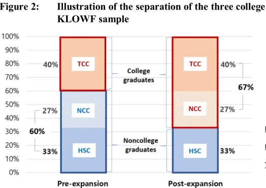
To identify HSC, NCC, and TCC from the sample, I rely on the assumption of monotonic expansion and the estimation of the probability of college completion. Three education classes are defined only counterfactually. The observed data suffer from the traditional problem of missing observations, as there is only one observation between the pre-expansion college decision (what one would do if she completed high school before the expansion) and the post-expansion college decision (what one would do if she completed high school after the expansion) for each individual. To resolve this problem, I construct the missing counterfactual college outcomes (e.g., what a pre-expansion woman would have chosen had she belonged to the post-pre-expansion cohort and what a post-expansion woman would have chosen had she been in the pre-expansion cohort) using the following procedure proposed by Choi (2015) for the estimation of college expansion effects on earnings and occupational status. I refer to Figure 2 for a visual illustration.
First, I assume a monotonic college expansion; no one changes her decision from college attendance to non-college attendance because of the expansion. This is a standard assumption in research examining heterogeneous responses (Imbens and Angrist 1994). Under this assumption, all college graduates in the pre-expansion period are assumed to be college graduates in the post-expansion period (TCC). Similarly, all non-college graduates in the post-expansion years are assumed to be non-college graduates in the pre-expansion period (HSC).
Second, to divide non-college graduates in the pre-expansion cohort into HSC and NCC and to divide the post-expansion college graduates into NCC and TCC, I utilize the estimation of predicted probability. First, I estimate the probabilities of a college education for the pre- and post-cohorts, respectively. I then compute their counterfactual probabilities using the estimated function of the other cohort such that:
= Λ( ) and = Λ( ),
where and denote the counterfactual probabilities of college completion for
pre-expansion women and post-expansion women, respectively,Λ(⋅) is the inverse logit function, and Z is a vector of pre-college covariates that predict college completion. Then, I assign pre-expansion non-college graduates with relatively higher counterfactual probabilities to NCC, assigning others to HSC. Likewise, post-expansion college graduates with higher counterfactual probabilities to TCC and those with lower probabilities to NCC (see Figure 2). I did this procedure probabilistically rather than deterministically, by incorporating randomness. More specifically, I simulate the counterfactual college outcome by randomly drawing a binary variable (0 or 1) using the calculated counterfactual probability as a Bernoulli parameter.5 In short, the NCC women are the combination of those who are less likely to go to college in the pre-expansion period but actually did go to college as post-pre-expansion women and those who did not go to college as pre-expansion woman but are more likely to go to college in the post-expansion period (see Appendix A for more specific details of this procedure).
I then estimate the pre-post difference in the transition rate of first marriage or first birth across these three groups using the difference-in-difference (DD) design in the
5 Here, I implicitly assume ignorability, which states that college-going can be perfectly predicted by the
discrete-time hazard rate model.6 The DD model predicting the discrete-time hazard rate of first marriage or first birth is expressed as follows:
= ( + + + + + +
+ + ),
where indicates the conditional probability of first marriage or first birth at time,t,A indicates age, Post indicates the post-expansion cohort, and X denotes a vector of control variables that are likely to affect the outcome between the pre- and post-expansion cohorts disproportionately for reasons other than college post-expansion. (⋅) is the inverse logit function because I use logit models following the popular standard for the discrete-time hazard analysis. and illustrate the pre-expansion levels of the hazard rate for NCC and TCC, respectively, relative to the reference group, HSC. illustrates the change in the hazard rate for HSC during the period of college expansion. In the DD design, is assumed to offer a common baseline trend that college classes would experience without the treatment of college expansion. This common trend assumption is the essential foundation to identifying the treatment effect with the estimated divergence from the common trend in the DD design (Angrist and Pischke 2009).
The interaction effect between NCC and post-expansion, , is the parameter of our primary interest. captures an additional change in the rate of transition to marriage or parenthood for NCC relative to HSC. This parameter reflects the total effect of college expansion that NCC women could experience due to the expansion, which is the sum of the quantity effect and the return effect. Another interaction effect, , is also a quantity of interest, as it captures the change in the hazard rate among TCC women compared with HSC women. By definition, this change is attributable to social changes that are not directly related to college expansion but that influence the events of family formation disproportionately differentially between college graduates and non-college women. Assuming that NCC women and TCC women share a common return effect, we can also identify the quantity effect from − .7, 8
6 As the procedure involves a simulation of a random drawing, I repeated the entire sequence of steps 100
times and averaged the estimated coefficients and standard errors as is done in the procedure of multiple imputation.
7 The validity of the assumption of common return effect is subject to empirical examination, considering
likely heterogeneity among college graduates. I address this issue as a robustness check in a later section.
8 Alternatively, − can be directly estimated by setting TCC as an omitted reference group instead of
4.3 Variables
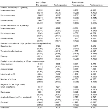
For the measures of college decisions, I consider two variables: whether or not a woman completed any type of college (2-year or 4-year) and whether she completed and attained a 4-year college degree. To predict the probability of college completion, I consider several precollege covariates that are commonly used for the estimation of returns to education, including parental education, parental occupation at age 15, self-evaluated economic status of her family at age 15, family structure at age 15, number of siblings, urban/rural residence at age 15, high school type, and birth year dummies. For parents’ education, I consider the highest level of father’s and mother’s education completed. I use mother’s education for those for whom father’s education is missing. For parental occupation, I consider four categories of father’s occupation or mother’s occupation if father’s occupation is missing or not available: (1) professional, managerial, and white-collar occupations, (2) sales and service occupations, (3) technicians, production workers, and laborers, and (4) farming and fishing occupations. For the family structure, I construct a dummy variable indicating whether a respondent lived with both parents at age 15. For high school type, I create a dummy variable indicating whether a respondent went to an academic high school (versus a vocational or art school).
For the outcomes of family formation, I examine age-specific patterns of first marriage and first childbirth. The reason I focus on first birth is that there are not sufficient observations in the KLOWF sample for second and subsequent births conditional on first or second birth. However, first childbirth is consequential, as it affects a woman’s total fertility (Spain and Bianchi 1996). The timing of first marriage is also consequential, especially in the South Korean context. As childbearing out of wedlock is very rare, a delay in first marriage is directly linked to a delay in first childbirth (Kye 2008). The risk sets range from age 18 to ages 30 to 36, depending on the birth year within each expansion cohort. I excluded a small number of women who experienced first marriage and first birth before age 18. Person-year observations are right-censored when age as the time indicator reaches the reported age at first marriage or childbirth.
first birth, by about a year, suggest that these substantial reductions in marriage and birth are not largely through delayed timing.
Table 1: Descriptive statistics
Pre-expansion cohort (1965–1971)
Post-expansion cohort (1976–1982)
College completion
No college 0.60 0.33
Junior college 0.11 0.26
4-year college+ 0.28 0.42
Marriage and childbirth
Ever-married at 30–36 0.92 0.75 Age at first marriagea 25.18 (3.45) 25.87 (2.99)
Ever had a child at 30–36 0.88 0.64 Age at first childbirthb 26.52 (3.83) 28.62 (3.78)
Pre-college covariates
Father’s education
<= primary 0.41 0.23
Lower-secondary 0.24 0.24 Upper-secondary 0.23 0.41 >= postsecondary 0.13 0.12 Mother’s education
<= primary 0.65 0.36
Lower-secondary 0.19 0.30 Upper-secondary 0.13 0.30 >= postsecondary 0.03 0.05 Parental occupation at 15
Professional/managerial/office 0.25 0.28
Sales/service 0.19 0.22
Technical/production/labor 0.18 0.28
Farming 0.37 0.22
Family’s economic standing (self-rated) at 15
Below average 0.28 0.23
About average 0.51 0.59
Above average 0.21 0.17
Intact family (lived with both parents) 0.92 0.91 Number of siblings 3.57 (1.60) 2.05 (1.21) Region at 15
Large cities 0.38 0.46
Small cities/towns 0.23 0.30
Rural areas 0.39 0.23
Attended general high school (vs. vocational) 0.63 0.62
Sample size (Proportion) 1140 (0.52) 1065 (0.48)
Notes: a. Only those who have been ever married; b. Only those who have had a child.
In general, there was an upgrade in family background measures across the cohorts. The parents of post-expansion cohort women have more education and are less likely to be farmers. On average, the post-expansion cohort women tend to have fewer siblings and grew up in urban areas more than did the pre-expansion cohort of women. As mentioned earlier, I adjusted for these differences between the cohorts by including the variables as controls. Their coefficients are omitted in the results but are available upon request.
5. Results
5.1 College expansion effects on age-specific transition rates of first marriage and first birth
Table 2 reports the DD estimates from the discrete-time hazard rate analysis of first marriage. The result shows that there is no statistical evidence of a gap in the rate of first marriage before the expansion between the three groups defined by college education and expansion. I find a weak and statistically insignificant difference between TCC and the other two college classes before the expansion. That is, the KLOWF sample suggests little or a very weak college gap in the transition to first marriage in the pre-expansion period.
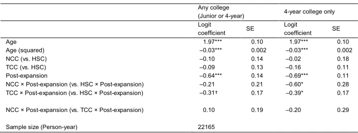
Table 2: Difference-in-difference estimates from the discrete-time hazard rate analysis of first marriage
Any college
(Junior or 4-year) 4-year college only Logit
coefficient SE Logitcoefficient SE Age 2.69*** 0.12 2.68*** 0.12 Age (squared) –0.05*** 0.002 –0.05*** 0.002 NCC (vs. HSC) –0.04 0.14 0.04 0.18 TCC (vs. HSC) –0.05 0.12 –0.15 0.11 Post-expansion –0.28† 0.15 –0.43*** 0.11 NCC × Post-expansion (vs. HSC × Post-expansion) –0.39† 0.21 –0.60* 0.28 TCC × Post-expansion (vs. HSC × Post-expansion) –0.42* 0.18 –0.34* 0.16
NCC × Post-expansion (vs. TCC × Post-expansion) 0.04 0.19 –0.26 0.29
Sample size (Person-year) 18280
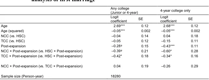
The coefficients of post-expansion show that the rate of first marriage dropped notably for all three educational classes. This decline in the baseline hazard rate is especially more remarkable when we look at the classes defined by the expansion of the 4-year university sector. The baseline odds of age-specific first marriage fell by 24% (e–0.28=0.76) and 35% (e–0.43=0.65), respectively, throughout college expansion. In addition to this fall, the estimates of the interaction effects between NCC and post-expansion, , indicate further significant reductions in the hazard rate of first marriage for the New College Class women, 32% (e–0.39=0.68, for junior or 4-year colleges) and 45% (e–0.6=0.55, for 4-year colleges only), in terms of odds. These quantities illustrate the total effect of college expansion. TCC shows a similar pattern. There are additional reductions in the odds of marriage transition by 34% (e–0.42=0.66, for junior and 4-year colleges) and 29% ( e–0.34=0.71 , for 4-year colleges only), respectively. These interaction effects, between TCC and post-expansion, provide the return effects of the expansion, . Although, I find no statistical evidence that the reduction in the hazard of first marriage was different between two college classes. As the gap between two college classes, − , indicates the quantity effect of college expansion, the results suggest that the substantial college expansion effect consisted of a small insignificant quantity effect and a large significant return effect. This pattern is generally similar to both types of college expansion.
Figure 3: The discrete time probabilities of first marriage and first birth
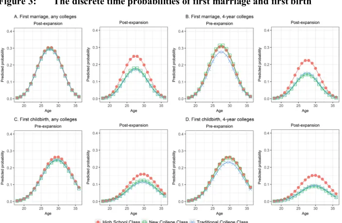
Table 3: Difference-in-difference estimates from the discrete-time hazard rate analysis of first birth
Any college
(Junior or 4-year) 4-year college only Logit
coefficient SE
Logit
coefficient SE Age 1.97*** 0.10 1.97*** 0.10 Age (squared) –0.03*** 0.002 –0.03*** 0.002 NCC (vs. HSC) –0.10 0.14 –0.02 0.18 TCC (vs. HSC) –0.09 0.13 –0.16 0.11 Post-expansion –0.64*** 0.14 –0.69*** 0.11 NCC × Post-expansion (vs. HSC × Post-expansion) –0.21 0.21 –0.60* 0.28 TCC × Post-expansion (vs. HSC × Post-expansion) –0.31† 0.17 –0.39* 0.17
NCC × Post-expansion (vs. TCC × Post-expansion) 0.10 0.19 –0.20 0.29
Sample size (Person-year) 22165
Notes: (1) All the models include college characteristics to control for the likely influences of the different distributions of the pre-college covariates between pre- and post-expansion cohorts. Their coefficients are omitted (available upon request). (2) The estimates are derived from 100 simulations. (3) Sampling weights are applied. ***: p < 0.001, **: p < 0.01, *: p < 0.05, †: p < 0.1.
Both NCC and TCC experienced additional declines in the likelihood of first birth; the odds of being a mother fell by 19% ( e–0.21=0.81 , for any type) to 45% (e–0.60=0.55, for 4-year) for NCC and by 27% (e–0.31=0.73, for any type) to 32% (e–0.39=0.68, for 4-year) for TCC. Most of those declines are statistically significant, except for the NCC women complying with the expansion of any type of college. Again, both differences in additional declines between the two college groups, − , are not statistically different from zero.
The lower panels of Figure 3 visually illustrate the three educational classes’ first birth rate. The peak rate of first birth is at age 30, which is considerably higher than the peak age of first marriage. Again, I find very small educational gaps in the transition to first birth before the expansion. However, the declines in the rate of first birth for the two college classes are notably larger than the decline for HSC women. The two college classes are not distinguishable, however. Figure 3, therefore, shows the graphical summary of how educational gradients in first marriage and first birth emerged throughout the period of college expansion. Overall, the analysis of first birth suggests that college expansion substantially affected the entry into motherhood for South Korean women mostly through the widening college gap in becoming a mother during the period of college expansion. The quantity effect is, again, small and not statistically measurable.
changes in marriage or by changes in first marital birth. In this analysis, the major time variable is years since first marriage. I also control for age.
Unlike previous analyses, I apply the inverse probability weight (IPW) to address a concern about an endogenous selection bias that comes from the collider problem (Elwert and Winship 2014). Marital status is a collider variable that is causally predicted by educational class and unobserved factors affecting the decision regarding motherhood. Conditioning on marital status, therefore, may generate an endogenous selection bias (See Appendix C for the more detailed illustration). The IPW, which is the inverse of the predicted probability of entry into first marriage, adjusts for the bias by blocking the causal path from educational class to first marriage (Elwert and Winship 2014; Robins, Hernán, and Brumback 2000). I use a stabilized version to reduce the sample variance (Robins, Hernán, and Brumback 2000):
=Pr (Pr (= 1| , ),= 1)
where the denominator is the predicted probability of first marriage conditional on pre-college characteristics and educational class, and the numerator is the unconditional probability of first marriage.9
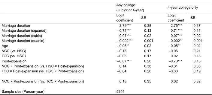
Table 4 shows the result. In comparison with the two previous results, two noteworthy patterns are found. First, the baseline decline in the first marital birth is significant and substantially larger than that in first marriage and unconditional first birth: 58% (=1– e–0.87, for any type) and 52% (=1–e–0.73, for 4-year colleges), in terms of odds. Second, no statistically significant deviance from the baseline reduction is detected for either college class. None of the total, return, or quantity effects are significantly large at the 95 and 90% confidence levels. The results of Table 4 suggest that the substantial decline in first marital birth can explain the country’s falling fertility rate. However, it is indifferent to education. I do not find evidence of the influence of college expansion on first marital birth (see the figure in Appendix E for the visual presentation of this result).
Comparing this result with the result from the analyses of unconditional first birth provides evidence that a growing educational difference in entry into first birth, alongside the college expansion effect, is mostly attributable to a change in entry into marriage rather than a change in marital fertility. This is generally consistent with prior research documenting that the current trend of very low fertility in South Korea was mainly driven by delayed marriage and a decrease in the proportion of married women rather than marital fertility (Lee 2012; Suzuki 2005).
Table 4: Difference-in-difference estimates from the discrete-time hazard rate analysis of first marital birth
Any college
(Junior or 4-year) 4-year college only Logit
coefficient SE
Logit coefficient SE Marriage duration 2.79*** 0.38 2.75*** 0.37 Marriage duration (squared) –0.73*** 0.13 –0.71*** 0.13 Marriage duration (cubic) 0.07*** 0.02 0.07*** 0.02 Marriage duration (quartic) –0.002*** 0.001 –0.002** 0.001 Age –0.05** 0.02 –0.05** 0.02 NCC (vs. HSC) –0.18 0.17 –0.06 0.21 TCC (vs. HSC) –0.06 0.17 0.02 0.13 Post-expansion –0.87*** 0.20 –0.73*** 0.13 NCC × Post-expansion (vs. HSC × Post-expansion) 0.14 0.38 –0.31 0.30 TCC × Post-expansion (vs. HSC × Post-expansion) –0.04 0.20 –0.33 0.19
NCC × Post-expansion (vs. TCC × Post-expansion) 0.18 0.35 0.02 0.32
Sample size (Person-year) 5844
Notes: (1) All the models include college characteristics to control for the likely influences of the different distributions of the pre-college covariates between pre- and post-expansion cohorts. Their coefficients are omitted (available upon request). (2) The estimates are derived from 100 simulations. (3) Sampling weights and inverse probability weights are applied. ***: p < 0.001, **: p < 0.01, *: p < 0.05, †: p < 0.1.
Table 5 summarizes how the total effect of college composition can be broken down into the quantity effect and the return effect, given that the assumption of the common return change holds. A consistent pattern regardless of the different specifications of treatment and outcomes is a significantly large negative effect of college expansion on the odds of family formation outcomes, ranging from –45% (4-year college, first marriage, and first birth) to –19% (any college, first birth), with a dominant role of the return effect, which ranges from –34% (any college, first marriage) to –27% (any college, first birth). The quantity effect is positive and small for the expansion of any type of college. For the expansion of 4-year colleges, we can see slightly larger negative quantity effects, but they are also short of statistical significance.
Table 5: The summary of college expansion effects on the odds of first marriage and first birth
Any college (Junior or 4-year) 4-year college
First marriage First birth First marriage First birth Δ sig. Δ sig. Δ sig. Δ sig. Total effect –32% † –19% –45% * –45% * Quantity effect 2% 8% –14% –13% Return effect –34% * –27% † –29% * –32% *
5.2 Unobserved heterogeneity
The findings documented in the previous section are justified only when two key identifying assumptions about unobserved heterogeneity are valid. First, I assumed that both college classes shared a common change in marriage and childbirth returns to college education after all the observed factors were conditioned. With this assumption, we could identify the quantity effect by simply subtracting the return effect ( ) from the total effect ( ). This is also necessary for the parallel trend assumption, an essential identifying assumption of the difference-in-difference model (Angrist and Pischke 2009). The second assumption is that college decisions are fully explained and predicted by the observed pre-college variables and that any possible effects of unobserved confounding factors are constant throughout the college expansion. Any selection bias due to unobserved pre-college factors affecting both college completion
and family outcomes do not bias the estimates of and . This assumption of
ignorability justifies the use of my random drawing simulation method. A key question then is whether NCC women are different in terms of unobserved characteristics from HSC and TCC women and how the differences affect the estimates. I address this question in two ways.
First, to investigate whether the two college classes share a common return change, I estimate the change in return to college education between pre-expansion and post-expansion as an interaction effect between post-post-expansion and college completion. The interaction is driven by the whole group of college graduates, including TCC and NCC, so any notable difference between the coefficient of the interaction and undermines the validity of the common return effect assumption. Conversely, if also represents the return change among NCC, we can expect an ignorable difference between the two coefficients. Table 6 reports the comparison of the coefficients. The two estimated coefficients are very similar with minuscule differences. This result convincingly
confirms that also represents the return effect of NCC and, therefore, −
captures the quantity effect.
Table 6: The price effects for traditional college class and all college graduates
Any college (Junior or 4-year) 4-year college TCC
× Post-expansion
College grads × Post-expansion
TCC
× Post-expansion
College grads × Post-expansion First marriage –0.42* –0.40* –0.34* –0.36* First birth –0.31† –0.30* –0.39* –0.41**
Note:**: p < 0.01, *: p < 0.05, †: p < 0.1.
introduce a randomly-simulated hypothetical variable that represents an unobserved confounding factor, U.U is designed to correlate with college completion and family
outcomes. My strategy is to examine how and change according to the varying
correlations of U with college completion and with the outcomes. The hypothetical variable U may be an indicator of some unobserved ability or aspirations, which can affect both educational attainment and family outcomes (Upchurch, Lillard, and Panis 2002). To learn what correlations of U with college and family formation events are empirically plausible, I estimate those correlations utilizing an external data source.10 The plausible correlations between U and college completion are 0.2 to 0.25 for any college and 0.4 and 0.45 for 4-year colleges. The correlations betweenU and the family outcomes range from –0.1 to –0.15. These ranges constitute empirically realistic ranges of correlations over which we should pay attention to the changes in and .
Figure 4 show how and vary over the correlation estimates between U and college completion whenU is incorporated in the analysis. For a readable presentation, I fix the correlations between U and marriage and between U and childbirth to –.2, the reasonable upper bound of the correlations. The result shows that the estimated values of are very robust toU in all analyses. The values of are relatively less robust to the presence of unobserved heterogeneity in the case of first marriage (but not for first birth). The significantly negative coefficients of in the marriage analyses become much closer and not statistically different from zero once U is introduced.11 These patterns suggest two findings. First, the issue of unobserved confounding appears to be negligible for the effects on first birth. Second, the return effects on first marriage are robust to unobserved confounding, but any negative but statistically insignificant quantity effects may be positive when considering the presence of omitted confounders. In any case, however, those quantity effects are highly likely to be small and insignificant.
10 To calculate the empirical correlations, I utilize data from the Korean Labor and Income Panel Study
(KLIPS). I illustrate the details of the procedure in Appendix D.
11 The coefficients of this robustness analysis are overestimated becauseU is designed to be uncorrelated with
Figure 4: The estimated coefficients under varying scenarios of the hypothetical confounder
Note: (1) The correlations of the hypothetical confounder,U, with marriage and first birth are set to –0.2, which is an empirically realistic correlation drawing from the KLIPS data. (2)b denotes the originally reported coefficients without controlling forU as reported in Tables 3 and 4. (3) Whiskers demonstrate 95% confidence intervals.
an alternative. In this matching approach, we lose some unmatched observations but can check sensitivity to the regression assumptions, such as the imposition of a parametric functional form and extrapolation. The analyses from CEM do not yield substantively different results, suggesting the general robustness of the findings to pre-post differences other than the expansion. I report the details of this robustness check in Appendix F.
To summarize, the auxiliary analyses suggest that can be taken as a good indicator of the return effects that NCC women could also experience. A minimal or limited role of the unobserved factors in the estimation of college expansion effects is also suggested. The most robust finding across all of the analyses is the significantly large negative return effect of college expansion, a decrease in the odds of transition to first marriage or first birth by more than 30%.
6. Conclusion and discussion
In this study, I examine how the large-scale college expansion in South Korea affected the probability of entering a first marriage and first birth, focusing on pre-post differences among NCC women relative to those among women in the TCC and HSC. The results from the discrete-time hazard models and a set of auxiliary analyses suggest that college expansion played a significant role in the declines in first marriage and first birth, but the effects are predominantly explained through changing educational gradients (the return effect) rather than by NCC women’s increased quantity of education (the quantity effect). These findings suggest that a major route through which college expansion contributed to the fertility decline in South Korea was its interactions with other important social changes. Without those other changes, college expansion per se would not have affected the family formation outcomes. In addition, I do not find evidence of significant differences between education classes in the changes in first marital birth. This implies that the college expansion effect on fertility worked indirectly, through entry into marriage. Similar coefficients between the models of any college and 4-year colleges suggest that the result was largely driven by the expansion of 4-year colleges rather than by junior colleges. Finally, the robustness checks confirm that the findings are not sensitive to the assumptions upon which my analysis relies.
and childbearing might differ across educational groups. Prior research reports that the fertility rate of college-educated women is more likely to recuperate later, suggesting that they tend to postpone, rather than avoid, childbearing (Martin 2000; Rindfuss, Morgan, and Swicegood 1988). However, this recovery has not been found in marriage among high-educated South Korean women (Choe and Li 2010; Park, Lee, and Jo 2013; Woo 2009; Yoo 2016). The possibility that the currently estimated college expansion effects are moderated by a recuperation mechanism at the end of the fertility age among post-expansion women needs to be explored in further research.
Second, this study considers only first childbirth. As mentioned earlier, first birth is consequential for later fertility decisions and the outcomes of higher-order parities (Spain and Bianchi 1996), but a fertility decline also can be driven by changes at higher-order parities rather than an increase in childless women. Suzuki (2008) demonstrated that the largest decline in fertility in South Korea between 2000 and 2005 occurred at the parity progression from one to two. In this vein, evidence of this study should be considered as suggestive rather than conclusive when an implication for total fertility is drawn.
The central findings of this paper raise three important issues for further discussion. First, the small and insignificant quantity effects on first marriage and first birth suggest that the rising level of women’s educational attainmentper se might not be a meaningful contributor to the country’s lowest-low fertility. This finding appears to disagree with prior research identifying women’s upgraded education as a major factor leading to lowest-low fertility (Billari 2008; Frejka, Jones, and Sardon 2010; Jones 2007; Kohler, Billari, and Ortega 2002). However, it also resonates with more recent causal evidence from the UK data that the observed association between women’s increased level of education and the postponement of first birth is largely explained by selection, in particular by family background factors (Tropf and Mandemakers 2017). The findings of this paper also suggest that the marginal group of the Korean college expansion, largely defined by pre-college family background factors, does not show significant differences in changes in first marriage and childbirth. This leads us to a skeptical view on the causal effect of educational expansion on marriage and especially childbirth.
women’s college education across low fertility societies suggests a weak association between college expansion and fertility. Indeed, researchers have emphasized that the associations between educational expansion and family outcomes are contingent on various institutional contexts of the given society, such as labor markets (Adserà 2004), life course (Billari 2008; Billari and Kohler 2004), welfare and childcare (Jones 2007; Rindfuss, Morgan, and Offutt 1996; Suzuki 2008), housing (Mulder and Billari 2010), and education (Anderson and Kohler 2013; Jones 2007). Frejka and colleagues apply this to the East Asian lowest-low fertility: “Rising education of women has played a key role in the very low fertility reached in East Asia. Yet it is not the high level of education per se that is important…Rather, it is the extraordinarily rapid expansion of education in the East Asian institutional context that is the key” (Frejka, Jones, and Sardon 2010: 597).
This discussion provides an important ground for further policy implications: for countries that have achieved the high levels of economic and social development, increasing women’s education does not necessarily bring a fertility decline. Rather, recent cross-national evidence suggests that in the context of advanced societies, increases in women’s empowerment and human capital are associated with higher fertility (Myrskylä, Kohler, and Billari 2009). This view suggests that we need to consider educational expansion, especially in higher education, as a factor that may promote fertility rather than blame it for fertility declines. This notion highlights the need for a radical shift in social and population policies when a country reaches a certain level of socioeconomic development. To promote fertility, policymakers should abandon efforts to constrain women to more traditional roles in the family as primary caregivers. Instead, policy efforts to empower women to successfully manage their roles in both the workplace and the family are imperative. It should also be noted, however, that educational expansion is a necessary but probably insufficient condition for women’s entitlement and empowerment.
crisis, however, undermined the economic capabilities of many middle-class families and increased the real and psychological costs of marriage for these families. I speculate that the changes in economic conditions triggered a change in strategies and preferences about marriage timing and childbearing and that this was relatively stronger for college-educated and middle-class women.
Second, an economic crisis yields many uncertainties among young adults about their future careers and induces a diverging calculation of the opportunity costs of parenthood across educational groups (Sobotka, Skirbekk, and Philipov 2011). For college graduates, increasing career uncertainty increases the perceived costs of sacrificing a career for children and leads to greater risk-aversion (McDonald 2002; Sobotka, Skirbekk, and Philipov 2011). For many non-college graduates with precarious employment positions, the perceived change in the costs of sacrificing a career for parenthood is not as large as for college graduates. The risk aversion, therefore, does not motivate non-college graduates to delay or avoid parenthood as it does college graduates. Rather, poor economic conditions may make parenthood a more attractive and justifiable option for less-educated women (Friedman, Hechter, and Kanazawa 1994; Sobotka, Skirbekk, and Philipov 2011). This prediction has been confirmed by previous research in the context of the South Korean economic crisis (Park, Kim, and Kim 2005; Lee 2006).
An economic crisis, however, cannot fully explain the persistence of lowest-low fertility in a society. If the economy recovers but the very low fertility does not, the sustained lowest-low fertility requires another explanation (Goldstein, Sobotka, and Jasilioniene 2009), and South Korea presents such a case. Total fertility fell below 1.3 for the first time in 2001, which was immediately after the economic crisis and the subsequent recession. Macroeconomic indicators show a relatively quick and clear economic bounce-back, but total fertility has remained at the lowest-low level. Existing research presents two explanations. First, mechanisms generating looping traps have been considered. Fertility-related behaviors resulting from certain initial factors (e.g., the economic crisis) can become new norms or values that remain firm even after those initial causal factors disappear, and the new norms or values reinforce such behaviors that keep fertility very low (Lutz 2008; Lutz, Skirbekk, and Testa 2006). Second, researchers also emphasize the institutional factors in which lowest-low fertility is rooted (McDonald 2006). Unless effective pro-natal policies reform those institutions successfully, a recovery from the economic crisisper se does not guarantee a rebound of fertility. Moreover, the looping traps and resistant institutional settings are likely to intertwine and reinforce the tendency to keep fertility low.
References
Adserà, A. (2004). Changing fertility rates in developed countries: The impact of labor market institutions.Journal of Population Economics 17(1): 17–43.doi:10.1007/ s00148-003-0166-x.
Ahn, N. and Mira, P. (2001). Job bust, baby bust?: Evidence from Spain. Journal of Population Economics 14(3): 505–521.doi:10.1007/s001480100093.
Anderson, T. and Kohler, H.-P. (2013). Education fever and the East Asian fertility puzzle. Asian Population Studies 9(2): 196–215. doi:10.1080/17441730.2013. 797293.
Angrist, J.D. and Pischke, J.-S. (2009).Mostly harmless econometrics: An empiricist’s companion. Princeton: Princeton University Press.
Becker, G.S. (1991).A treatise on the family. Cambridge: Harvard University Press. Billari, F.C. (2005). Europe and its fertility: From low to lowest low.National Institute
Economic Review 194(1): 56–73.doi:10.1177/0027950105061496.
Billari, F.C. (2008). Lowest-low fertility in Europe: Exploring the causes and finding some surprises.The Japanese Journal of Population 6(1): 2–18.
Billari, F.C. and Kohler, H.-P. (2004). Patterns of low and lowest-low fertility in
Europe. Population Studies 58(2): 161–176. doi:10.1080/0032472042000213
695.
Black, S.E., Devereux, P.J., and Salvanes, K.G. (2008). Staying in the classroom and out of the maternity ward? The effect of compulsory schooling laws on teenage births. The Economic Journal 118(530): 1025–1054. doi:10.1111/j.1468-0297. 2008.02159.x.
Blossfeld, H.-P. (1995).The new role of women: Family formation in modern societies. Boulder: Westview Press.
Blossfeld, H.-P. and Huinink, J. (1991). Human capital investments or norms of role transition? How women’s schooling and career affect the process of family formation.American Journal of Sociology 97(1): 143–168.doi:10.1086/229743. Brand, J.E. and Davis, D. (2011). The impact of college education on fertility: Evidence
Brewster, K.L. and Rindfuss, R.R. (2000). Fertility and women’s employment in industrialized nations. Annual Review of Sociology 26: 271–296. doi:10.1146/ annurev.soc.26.1.271.
Caldwell, J.C. (1980). Mass education as a determinant of the timing of fertility decline. Population and Development Review 6(2): 225–255.doi:10.2307/1972729. Choe, M.K. and Li, L. (2010). Estimating the effects of education on later marriage and
less marriage in South Korea: An application of a mixture survival model with proportional piecewise constant hazards. Journal of Applied Statistical Science 18(4): 553–567.
Choe, M.K. and Retherford, R.D. (2009). The contribution of education to South Korea’s fertility decline to ‘lowest-low’ level. Asian Population Studies 5(3): 267–288.doi:10.1080/17441730903351503.
Choi, S. (2015). When everyone goes to college: The causal effect of college expansion on earnings.Social Science Research 50: 229–245.doi:10.1016/j.ssresearch.20 14.11.014.
Cleland, J. (2001). Potatoes and pills: An overview of innovation-diffusion contributions to explanations of fertility decline. In: Casterline, J.B. (ed.). Diffusion processes and fertility transition: Selected perspectives. Washington, D.C.: National Academies Press: 39–65.
Cleland, J. and Wilson, C. (1987). Demand theories of the fertility transition: An iconoclastic view. Population Studies 41(1): 5–30. doi:10.1080/003247203100 0142516.
Elwert, F. and Winship, C. (2014). Endogenous selection bias: The problem of conditioning on a collider variable. Annual Review of Sociology 40(1): 31–53.
doi:10.1146/annurev-soc-071913-043455.
Frejka, T., Jones, G.W., and Sardon, J.-P. (2010). East Asian childbearing patterns and
policy developments. Population and Development Review 36(3): 579–606.
doi:10.1111/j.1728-4457.2010.00347.x.
Friedman, D., Hechter, M., and Kanazawa, S. (1994). A theory of the value of children. Demography 31(3): 375–401.doi:10.2307/2061749.
Goldin, C. and Katz, L.F. (2008). The race between education and technology. Cambridge: Harvard University Press.
Goldstein, J.R., Sobotka, T., and Jasilioniene, A. (2009). The end of “lowest-low” fertility? Population and Development Review 35(4): 663–699. doi:10.1111/ j.1728-4457.2009.00304.x.
Gustafsson, S. (2001). Optimal age at motherhood: Theoretical and empirical considerations on postponement of maternity in Europe. Journal of Population Economics 14(2): 225–247.doi:10.1007/s001480000051.
Happel, S.K., Hill, J.K., and Low, S.A. (1984). An economic analysis of the timing of childbirth. Population Studies 38(2): 299–311.doi:10.1080/00324728.1984.104 10291.
Iacus, S.M., King, G., and Porro, G. (2012). Causal inference without balance checking: Coarsened exact matching. Political Analysis 20(1): 1–24. doi:10.1093/pan/ mpr013.
Imbens, G.W. and Angrist, J.D. (1994). Identification and estimation of local average treatment effects.Econometrica 62(2): 467–475.doi:10.2307/2951620.
Jones, G.W. (2007). Delayed marriage and very low fertility in pacific Asia.Population and Development Review 33(3): 453–478. doi:10.1111/j.1728-4457.2007.001 80.x.
Kohler, H.-P., Billari, F.C., and Ortega, J.A. (2002). The emergence of lowest-low fertility in Europe during the 1990s.Population and Development Review 28(4): 641–680.doi:10.1111/j.1728-4457.2002.00641.x.
Kravdal, Ø. and Rindfuss, R.R. (2008). Changing relationships between education and fertility: A study of women and men born 1940 to 1964.American Sociological Review 73(5): 854–873.doi:10.1177/000312240807300508.
Kye, B. (2008). Delay in first marriage and first childbearing in Korea: Trends in educational differentials [electronic resource]. Los Angeles: California Center for Population Research.https://escholarship.org/uc/item/0x58f1p5.
Lee, C. (2012). A decomposition of decline in total fertility rate in Korea: Effects of changes in marriage and marital fertility. Korea Journal of Population Studies 35(3): 117–144.
Lee, S.Y. (2006). Economic crisis and the lowest-low fertility. Korea Journal of Population Studies 29(3): 111–137.
Lesthaeghe, R. (2010). The unfolding story of the second demographic transition. Population and Development Review 36(2): 211–251.doi:10.1111/j.1728-4457. 2010.00328.x.
Lutz, W. (2008). Has Korea’s fertility reached the bottom?Asian Population Studies 4(1): 1–4.doi:10.1080/17441730801963110.
Lutz, W., Skirbekk, V., and Testa, M.R. (2006). The low-fertility trap hypothesis: Forces that may lead to further postponement and fewer births in Europe.Vienna Yearbook of Population Research 4: 167–192.
Martin, S.P. (2000). Diverging fertility among US women who delay childbearing past age 30.Demography 37(4): 523–533.doi:10.1353/dem.2000.0007.
McDonald, P. (2002). Sustaining fertility through public policy: The range of options. Population 57(3): 417–446.doi:10.2307/3246634.
McDonald, P. (2006). Low fertility and the state: The efficacy of policy. Population and Development Review 32(3): 485–510. doi:10.1111/j.1728-4457.2006.0013 4.x.
Mills, M., Rindfuss, R.R., McDonald, P., and te Velde, E. (2011). Why do people
postpone parenthood? Reasons and social policy incentives. Human
Reproduction Update 17(6): 848–860.doi:10.1093/humupd/dmr026.
Monstad, K., Propper, C., and Salvanes, K.G. (2008). Education and fertility: Evidence from a natural experiment. Scandinavian Journal of Economics 110(4): 827– 852.doi:10.1111/j.1467-9442.2008.00563.x.
Mulder, C.H. and Billari, F.C. (2010). Homeownership regimes and low fertility. Housing Studies 25(4): 527–541.doi:10.1080/02673031003711469.
Myrskylä, M., Kohler, H.-P., and Billari, F.C. (2009). Advances in development reverse fertility declines.Nature 460(7256): 741–743.doi:10.1038/nature08230.
Neels, K., Murphy, M., Ní Bhrolcháin, M., and Beaujouan, É. (2014). Further estimates of the contribution of rising educational participation to fertility postponement: A model-based decomposition for the UK, France, and Belgium. Paper presented at Population Association of America 2014 Annual Meeting, Boston, Massachusetts, May 1–3, 2014.
Ní Bhrolcháin, M. and Beaujouan, É. (2012). Fertility postponement is largely due to rising educational enrolment. Population Studies 66(3): 311–327. doi:10.1080/ 00324728.2012.697569.
Ono, H. (2007). Does examination hell pay off ? A cost-benefit analysis of ‘Ronin’ and college education in Japan. Economics of Education Review 26(3): 271–284.
doi:10.1016/j.econedurev.2006.01.002.
Park, H., Lee, J.K., and Jo, I. (2013). Changing relationships between education and marriage among Korean women.Korean Journal of Sociology 47(3): 51–76. Park, K.-S., Kim, Y.-H., and Kim, H.-S. (2005). Main causes of delayed marriage
among Korean men and women: Contingent joints of status homogamy, gender role divisions, and economic restructuring.Korea Journal of Population Studies 28(2): 33–62.
Raymo, J.M., Park, H., Xie, Y., and Yeung, W.J. (2015). Marriage and family in East
Asia: Continuity and change. Annual Review of Sociology 41(1): 471–492.
doi:10.1146/annurev-soc-073014-112428.
Rindfuss, R.R. and Brauner-Otto, S.R. (2008). Institutions and the transition to adulthood: Implications for fertility tempo in low-fertility settings. Vienna Yearbook of Population Research 2008: 57–87.doi:10.1553/populationyearbook 2008s57.
Rindfuss, R.R., Morgan, S.P., and Offutt, K. (1996). Education and the changing age
pattern of American fertility: 1963–1989. Demography 33(3): 277–290.
doi:10.2307/2061761.
Rindfuss, R.R., Morgan, S.P., and Swicegood, G. (1988). First births in America: Changes in the timing of parenthood. Berkeley: University of California Press. Robins, J.M., Hernán, M.Á., and Brumback, B. (2000). Marginal structural models and
Silles, M.A. (2011). The effect of schooling on teenage childbearing: Evidence using changes in compulsory education laws.Journal of Population Economics 24(2): 761–777.doi:10.1007/s00148-010-0334-8.
Skirbekk, V., Kohler, H.-P., and Prskawetz, A. (2004). Birth month, school graduation,
and the timing of births and marriages. Demography 41(3): 547–568.
doi:10.1353/dem.2004.0028.
Sobotka, T., Skirbekk, V., and Philipov, D. (2011). Economic recession and fertility in
the developed world. Population and Development Review 37(2): 267–306.
doi:10.1111/j.1728-4457.2011.00411.x.
Spain, D. and Bianchi, S. (1996). Balancing act: Motherhood, marriage, and
employment among American women. New York: Russell Sage Foundation. Suzuki, T. (2005). Why is fertility in Korea lower than in Japan?Journal of Population
Problems 61(2): 23–39.
Suzuki, T. (2008). Korea’s strong familism and lowest-low fertility. International Journal of Japanese Sociology 17(1): 30–41. doi:10.1111/j.1475-6781.2008. 00116.x.
Tropf, F.C. and Mandemakers, J.J. (2017). Is the association between education and fertility postponement causal? The role of family background factors. Demography 54(1): 71–91.doi:10.1007/s13524-016-0531-5.
Upchurch, D.M., Lillard, L.A., and Panis, C.W.A. (2002). Nonmarital childbearing: Influences of education, marriage, and fertility. Demography 39(2): 311–329.
doi:10.1353/dem.2002.0020.
Waite, L.J., Goldscheider, F.K., and Witsberger, C. (1986). Nonfamily living and the
erosion of traditional family orientations among young adults. American
Sociological Review 51(4): 541–554.doi:10.2307/2095586.
Woo, H. (2009). The impact of educational attainment on first marriage formation: Marriage delayed or marriage forgone? Korea Journal of Population Studies 32(1): 25–50.
Yoo, S.H. (2014). Educational differentials in cohort fertility during the fertility
transition in South Korea. Demographic Research 30(53): 1463–1494.
doi:10.4054/DemRes.2014.30.53.
Yoo, S.H. (2016). Postponement and recuperation in cohort marriage: The experience
of South Korea. Demographic Research 35(35): 1045–1078. doi:10.4054/Dem
Appendix A
The procedure of predicting the counterfactual college outcome (a more detailed illustration)
To produce effective predictions about what decision a woman in the pre- or post-expansion cohort would make on college-going if she belonged to the post- or pre-expansion cohort, I used the following steps.
1. Assuming the monotonicity of the South Korean college expansion (no one changes their decision from college attendance to non-college attendance as a result of the expansion), I assumed that all pre-expansion college graduates would be college graduates if they belonged to the expansion cohort (TCC). Similarly, all post-expansion non-college graduates would be non-college graduates if they belonged to the pre-expansion cohort (HSC).
2. In order to divide non-college graduates in the pre-expansion cohort into HSC and NCC, I used an estimation predicting the college outcome for the post-expansion cohort. More specifically, I used the logit model that predicts whether a woman completes college or not for the post-expansion cohort women to learn the function that would predict the probability of college completion in the post-expansion period:
= Λ ,
where denotes the probability of college completion for post-expansion women, Λ(⋅) is the inverse logit function, and is a vector of post-expansion women’s pre-college covariates that predict pre-college completion. I used this information to calculate the counterfactual probability of college completion for pre-expansion women, which shows the probability that a pre-expansion woman would have if she were a post-expansion woman as follows:
= Λ ,
where denotes the counterfactual probability of college completion for
pre-expansion women and is a vector of pre-expansion women’s characteristics that predict college completion.