DEMOGRAPHIC RESEARCH
A peer-reviewed, open-access journal of population sciences
DEMOGRAPHIC RESEARCH
VOLUME 39, ARTICLE 37, PAGES 991–1008
PUBLISHED 26 OCTOBER 2018
http://www.demographic-research.org/Volumes/Vol39/37/ DOI: 10.4054/DemRes.2018.39.37
Formal Relationship 28
Life lived and left: Estimating age-specific
survival in stable populations with unknown
ages
James W. Vaupel
Francisco Villavicencio
c
2018 James W. Vaupel & Francisco Villavicencio.
This open-access work is published under the terms of the Creative Commons Attribution 3.0 Germany (CC BY 3.0 DE), which permits use, reproduction, and distribution in any medium, provided the original author(s) and source are given credit.
1 Relationship 992
2 Proof 992
3 Related results 993
3.1 The stable population model 994
3.2 Life lived and left in stationary populations 995 3.3 The population of France from a life left perspective 997
4 Application 997
4.1 Life lived and left in a discrete-time framework 998 4.2 Example of application with simulated data 1000 5 The 1805 cohort life table of Swedish females 1002
5.1 Estimation of the growth rate 1003
5.2 Reconstruction of the survival curve 1003
6 Discussion 1005
Life lived and left: Estimating age-specific survival in stable
populations with unknown ages
James W. Vaupel1 Francisco Villavicencio2
Abstract
BACKGROUND
Demographers sometimes observe remaining lifespans in populations of individuals of unknown age. Such populations may have an age structure that is approximately stable. To estimate life tables for these populations, it is useful to know the relationship between the number of individuals at a given agea, and the number of individuals that are expected to dieatime units after observation. This result has already been described for stationary populations, but here we extend it to stable populations.
RESULTS
In a stable population, the population at a given ageais a simple function of the num-ber of deaths at remaining lifespana, the number of deaths at remaining lifespansaand higher, and the population growth rate. This property, which can be useful when ages are unknown, but individuals are followed until death, permits estimation of the under-lying unknown survival schedule of the population and calculation of the usual life table functions and statistics, including the stable age structure.
CONTRIBUTION
The main contribution of this article is to provide a formal proof of the relationship be-tween life lived and life left in stable populations. We also discuss the challenges of applying theoretical relationships to empirical data, especially due to the fact that in real-world applications time is not continuous and some adjustments are necessary to move from a continuous to a discrete-time framework. Two applications, one with simulated data and a second with Swedish data from the 19thcentury, illustrate these ideas.
1Interdisciplinary Center on Population Dynamics, University of Southern Denmark, Odense, Denmark.
Email:[email protected].
2Interdisciplinary Center on Population Dynamics, University of Southern Denmark, Odense, Denmark.
1. Relationship
Consider a stable population with constant growth raterthat is first observed at timet. LetN(a,t)be the unknown number of individuals in this population at any agea. Let
e
D(a,t)be the number of individuals in the population at timetwho dieatime units after first observation. These are the individuals at timetwho have exactlyatime units of life left. The term ‘life left’ pertains to the remaining lifetime until death, as opposed to ‘life lived’ or age of an individual or cohort.3 Let
e
N(a,t) = R∞
a De(x,t)dx: This function
gives the number of individuals from the initial population who are still alive at timet+a. Then, we have that
(1*) N(a,t+a) =De(a,t) +rNe(a,t),
whereN(a,t+a)is the number of individuals at ageaat time t+a.4 Furthermore, given a population in which ages are unknown but individuals are followed until death, this result can be used to derive the underlying unknown cohort survival schedule,
(2*) `(a) =N(a,t+a)
N(0,t) =
e
D(a,t) +rNe(a,t)
e
D(0,t) +rNe(0,t)
.
2. Proof
Stable population theory implies that
e D(x,t) =
Z ∞
0
B(t)e−rad(a+x)da=
Z ∞
x
B(t)e−r(a−x)d(a)da,
whereB(t)are the births at timetandd(a+x)is the unconditional risk of death at age
a+x. Applying the Leibniz rule for differentiation under the integral sign, we get
d
dxDe(x,t) = d dx
Z ∞
x
B(t)e−r(a−x)d(a)da= lim
M→∞
d dx
Z M
x
B(t)e−r(a−x)d(a)da
=−B(t)d(x) + lim
M→∞r
Z M
x
B(t)e−r(a−x)d(a)da
=−B(t)d(x) +rDe(x,t),
3Other terms such as ‘time-to-death,’ ‘remaining lifespan,’ ‘follow-up duration,’ or ‘residual life’ are also
frequently used to refer to life left.
and, rearranging terms,
(3) B(t)d(x) =− d
dxDe(x,t) +rDe(x,t).
Because`(a) =Ra∞d(x)dxfor alla≥0, integrating both sides of (3) yields
B(t)`(a) =
Z ∞
a
− d
dxDe(x,t) +rDe(x,t)dx
= lim
M→∞
Z M
a
−d
dxDe(x,t)dx+r
Z ∞
a e
D(x,t)dx
=− lim
M→∞De(M,t) +De(a,t) +rNe(a,t)
=De(a,t) +rNe(a,t).
Since`(a)is the probability of surviving from birth to ageaandB(t)are the births at timet, it follows thatB(t)`(a) = N(a,t+a), the population at ageaat timet+a, which proves (1*). Equation (2*) follows directly from (1*) and the definition of the cohort survival function`(a).
3. Related results
The main result in (1*) that describes the relationship between life lived and life left in stable populations has already been proved for the particular case of stationary popula-tions with growth rater= 0(Brouard 1989; Vaupel 2009; Villavicencio and Riffe 2016). To our knowledge, Vaupel was the first to generalize it to stable populations in an unpub-lished manuscript from 2013. Here we polish Vaupel’s proof and include some additional material.
In the stable population model, the crude birth rateband the crude death ratedare assumed to be constant over time, which permits estimation of the constant growth rater
of the population. LetN(t),B(t)andD(t)denote, respectively, the population size, the number of births, and the number of deaths at timetin a stable population. Then
(4) r=b−d= B(t)
N(t)−
D(t)
N(t),
and
(5) B(t) =D(t) +r N(t).
Equation (5) can be re-expressed as follows: In stable populations, at any timet
0 life left (deaths), plus an extra term that only depends on the constant growth rate and the population size. Equation (1*) extends this relationship to estimate the number of individuals at older ages when the ages are unknown but there is information about the remaining time until death. In population biology, for instance, one may think of a wild population that is captured at a certain time point, and then the deaths and the number of individuals that are still alive at each subsequent time point are recorded until extinction. This information can be used to estimate the age-specific survival, provided that the assumption of stability is not overly distorting and that it is possible to estimate the population growth rater.
Equations (4) and (5) pertain to a population with an initial age of 0, but they can be generalized to apply to a population with any initial agea. Then, at timet,B(t)would be the number of individuals who are agea,D(t)the number of individuals who die at age
aand older, andN(t)the number of individuals alive at ageaand older. The growth rate
ralso pertains to the population above agea, but in the stable model thisris the same for the entire population. Hence, Equation (1*) can be viewed as a generalization of (5). Note thatN(0,t+ 0) =B(t)because the population at age 0 at timetequals the births at timet. Further, the individuals who at timethave 0 remaining lifetime are the deaths, and thereforeDe(0,t) =D(t). Finally, the individuals from the initial population at time twho are still alive att+ 0are the same, soNe(0,t) =N(t). As a result, (5) leads to (1*)
whena= 0:
B(t) =D(t) +r N(t) =⇒N(0,t) =De(0,t) +rNe(0,t).
3.1 The stable population model
In 1760 Leonhard Euler (1707–1783) was the first to formally describe the concept of a stable population, defined as a population closed to migration experiencing fixed age-specific death rates, and births that vary in geometric progression for a prolonged period of time (Euler 1970). Euler’s work remained rather unknown to the scientific commu-nity, and his ideas were published during subsequent decades and centuries by scholars who independently rediscovered them. The development of a fully articulated theory of stable populations was due to Alfred J. Lotka (1880–1949) in a series of more than 30 articles and a book,Th´eorie analytique des associations biologiques. This book was first published in two separate volumes in 1934 and 1939 and, surprisingly, not translated into English until 1998 (Lotka 1934, 1939, 1998).
In stable populations, the population size at timetis given by
N(t) =
Z ∞
0
N(a,t)da=
Z ∞
0
B(t)e−ra`(a)da
given age at timetisN(a,t) = e−raN(a,t+a). Therefore, our basic result (1*) can also be used to estimate the unknown age structure at initial timet,
(6*) c(a,t) =N(a,t)
N(t) =
e−raN(a,t+a)
N(t) =e
−ra De(a,t) +rNe(a,t) N(t) .
It may also be interesting to observe that (6*) is equivalent to a more common ex-pression for the proportion of the population at ageain terms of the birth rateb,
(7) c(a,t) =b e−ra`(a),
as stated by Lotka more than a century ago (Lotka 1907). Equation (7) implies that the population structure does not depend on time because the birth ratebis constant. Here, we use the notationc(a,t)to highlight that we refer to the age structure at the time of capture when the follow-up of the population starts. But in stable populations, the period age structure – as well as the cohort survival schedule – is constant over time, so one could simply writec(a).5
Although stability is an abstract mathematical concept resulting from the continu-ous operation of strong demographic assumptions over the long run, these restrictions have turned out to be serviceable in many applications. Stable population theory has been widely used in the study of human and nonhuman populations, especially when ac-curate data is incomplete or problematic, as discussed in the manualThe Concept of a Stable Population: Application to the Study of Populations of Countries with Incomplete Demographic Statistics(United Nations 1968). Even though perfect stability is rarely observed, this book argues that many populations around the world are ‘semi-stable’ or ‘quasi-stable,’ and possess some of the properties of the stable population model. Semi-stable refers to populations that have an unchanging age structure, whereas quasi-Semi-stable describes populations in which fertility remains unchanged and mortality improves grad-ually.
3.2 Life lived and left in stationary populations
In stationary populations, in addition to fixed age-specific death rates and closure to mi-gration, the birth flow is constant over time because of the growth rater = 0, which implies that, in the long run, the number of births equals the number of deaths and the population size remains constant. This approach is more restrictive than stability but can lead to new insights about population dynamics. Some of these insights pertain to the symmetries between life lived and life left. Kim and Aron (1989) – and later Goldstein
5For a general overview of the main properties of stable populations, see for instance Preston, Heuveline, and
(2009) – proved that the average age of a stationary population equals average remain-ing life expectancy, whereas Riffe (2015) addressed the equivalence between the force of mortality by age and the force of increment by life left. Moreover, stationary populations present a symmetry between their age composition and the distribution of remaining life-times. This relationship was first described by Brouard (1986, 1989), and was later inde-pendently formulated by James Carey and colleagues in the study of the survival patterns of captive and follow-up cohorts of medflies (M¨uller et al. 2004, 2007). Vaupel (2009) proved that in stationary populations of infinite size and in continuous time, the probabil-ity that a randomly selected individual is ageaequals the probability that an individual has exactlyatime left until death. Villavicencio and Riffe (2016) suggested an alternative proof for empirical and finite stationary populations in a discrete-time framework.
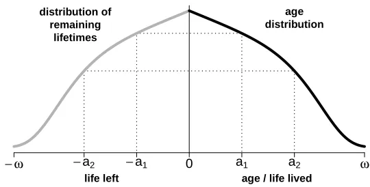
An alternative perspective is to consider the births and deaths in stationary popu-lations, which need to be continuously in balance to keep the population size constant. Hence, the number of individuals at age 0 (births) equals the number of individuals with 0 life left (deaths). Note that the first group forms a birth cohort, whereas in the second there are individuals from different ages who share the same time of death, forming a ‘death cohort.’ The key point is that this result is true for all ages when the population is stationary, meaning that the number of individuals at any ageaequals the number of individuals withalife left within the population. Figure 1 illustrates these ideas: Life left is plotted in the negative horizontal axis to convey the notion of a ‘countdown.’
Figure 1: Symmetries between the age composition and the distribution of
remaining lifetimes in stationary populations
− ω −a2 −a1 0 a1 a2 ω
age distribution distribution of
remaining lifetimes
age / life lived life left
Note: Parameterωrefers to the maximum observed lifespan.
and left because of the growth rater, but there is still a relationship between the age composition (captured byN(a,t)) and the distribution of remaining lifetimes (captured byDe(a,t)). Note that ifr= 0, thenN(a,t+a) =N(a,t)and (1*) becomes
N(a,t) =De(a,t).
This equivalence formalizes the concept of symmetry between life lived and left in sta-tionary populations that has just been described: The number of individuals agedaat timetequals the number of individuals who will die at timet+a.
3.3 The population of France from a life left perspective
Brouard (1986) presents an original overview of the population dynamics of France in the 20th century from a life left perspective. He compares the age structure of the French pop-ulation in several years with what he calls the ‘pyramide des ann´ees `a vivre,’ that is, the projected structure of remaining lifetimes of the cohorts alive in those years. He also in-troduces the concept of ‘g´en´eration de d´ec`es’ (death cohort) mentioned above. Especially relevant are the two pyramids from 1901, which show that the male population above age 70 is surprisingly close to the population that at that time had more than 70 years of life left and lived at least until 1970. Lower remaining lifetimes were caused by traumatic events such as the two world wars that increased mortality, but in general there is a fairly close symmetry between both pyramids. In contrast, in the case of women the improve-ments in mortality were more marked, and thus the pyramid of remaining lifetimes has more individuals with higher values, given that more women lived longer than 70 years after 1901 than those above age 70 in that year. Brouard concludes that the analysis of the remaining lifetimes offers a new interesting perspective for the study of population dynamics, notably for older ages. He suggests the estimation of life left according to some health markers, which could provide better insights into the characteristics of the old population and help in the assessment of proper policies.
4. Application
Demographers like to think of time as a continuous process, which permits the use of differential calculus and facilitates the proof of demographic relationships among demo-graphic functions. This has been the case in the statement and proof of (1*) and (2*), as well in the works mentioned above that are based on the stable population theory devel-oped by Lotka (1939).
noninteger – number of births and deaths at any time. On the contrary, in an empirical population in which individuals are indivisible, the instantaneous number of births and deaths would be zero, and the number of births and deaths would have to be computed in time intervals between observations. Villavicencio and Riffe (2016) adopted this ap-proach to provide an alternative proof of the symmetries between life lived and left in empirical stationary populations. This approach represents a more realistic setup, but has the disadvantage of making the demonstration more complex than in the continuous case.
4.1 Life lived and left in a discrete-time framework
In an empirical setup, some adjustments are necessary to adapt Equations (1*), (2*), and (6*) to a discrete-time framework. In general, we can only get the population counts at exact timest,t+ 1,t+ 2, etc., and we may not be able to know what births and deaths occurred between observations. Moreover, a slightly different notation is usually adopted to account for the fact that ages are not exact: In the following, we use subindices for the age variable to refer to the ‘age interval[a,a+ 1)’ instead of the ‘exact agea.’
Suppose a population is first captured at timetand the total number of individuals
N(t)is recorded. This same population is observed again at timet+ 1and the number of individuals still alive are recorded, obtainingNe1(t), the individuals from the initial
population who are alive at timet+ 1, all of them at age 1 and above. The assumption of stability implies
(8) N1+(t) =e−rNe1(t),
whereN1+(t)is the unknown number of individuals that at exact timetwere age 1 and
above. Equation (8) can be used to estimate the population at age[0, 1)at exact timet:
N0(t) =N(t)−N1+(t)
=Ne0(t)−e−rNe1(t),
given thatN(t) =Ne0(t), the population at age 0 and above at exact timet. Analogously,
N1(t+ 1) =Ne1(t)−N2+(t+ 1)
=Ne1(t)−e−rNe2(t),
whereN1(t+ 1)is the number of individuals at age[1, 2)at exact timet+ 1,N2+(t+ 1)
is the number of individuals at age 2 and above at exact time t+ 1, andNe2(t)is the
timet+ais
(9*) Na(t+a) =Nea(t)−e−rNea+1(t).
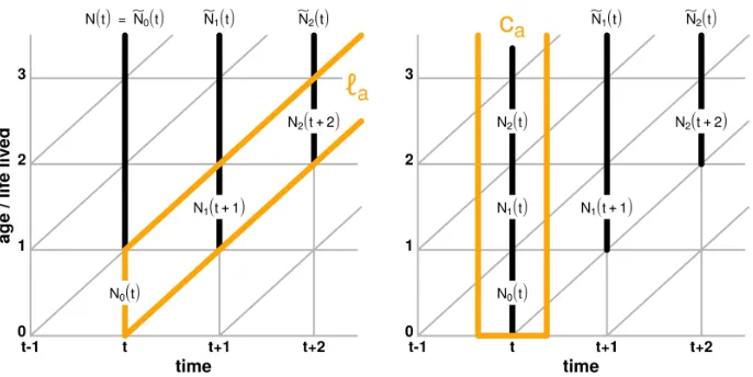
Equation (9*) is an extension of our basic result (1*) to the case of observations made not continuously but at points in timet,t+ 1,t+ 2, etc., and is valid for any time unit – minutes, hours, days, years, or decades. It is necessary, though, that the same unit is used to measure time and age, and that the population is observed at regular time points. The Lexis diagram in Figure 2 provides some intuition about these concepts and relationships.
Figure 2: Lexis diagram illustrating the relationship between life lived and life left in a discrete-time framework
t−1 t t+1 t+2
0 1 2 3
N0(t)
N1(t+1)
N2(t+2)
N(t)=N0(t) N1(t) N2(t)
N1+(t)
N2+(t+1)
e−r
e−r
e−r e−r
a
g
e / lif
e lived
time
Note: Life lived is captured byN(t),N0(t),N1(t+ 1), etc., and life left byNe0(t),Ne1(t),Ne2(t), etc. following
Equation(9*).
An equivalent expression to the survival schedule in (2*) for the discrete case follows immediately from (9*),
(10*) `a= Na(t+a)
N0(t)
= Nae (t)−e −r
e Na+1(t)
e
N0(t)−e−rNe1(t)
and the stable age structure defined in (6*) becomes
ca= Na(t)
N(t) =
e−raN a(t+a) N(t)
=e−raNae (t)−e
−r e Na+1(t)
N(t) . (11*)
Figure 3 illustrates these two last results in a Lexis diagram: By following a stable population with unknown ages from timet onward, and recording at each subsequent time step the number of remaining individuals alive (Ne0(t),Ne1(t),Ne2(t), etc.), we are
able to recover the cohort survival schedule`a(left panel) and the stable age structureca
(right panel).
Figure 3: Lexis diagrams illustrating the cohort survival schedule`a(left panel) and the stable age structureca(right panel) that can be estimated by following a stable population until extinction
Note: Stable population with unknown ages that is followed from timetonward, recording at each subsequent time step the number of remaining individuals alive, and applying(10*)and(11*).
4.2 Example of application with simulated data
we observe a population at regular time points until its extinction, and we record the
e
Na(t)values at each time step. Applying (9*), (10*), and (11*), we use these values to estimate the survival schedule used in the data simulation and the corresponding stable age structure. The R code (R Core Team 2018) to carry out this experiment is available in the supplementary materials; only a few details are provided below.
We adapt the same simplified example of a stable population used by Preston, Heuve-line, and Guillot (2001: 138–141), so the reader can refer to that book to find additional explanation. Suppose there is a hypothetical population in which all individuals die be-fore age 5, defined by the following life table:
Table 1: Life table (survival schedule) used in the data simulation
a 0 1 2 3 4 5
`a 1.00 0.60 0.40 0.20 0.05 0.00
Function `a gives the probability of surviving from age [0, 1)to age [a,a+ 1). All cohorts are driven by this survival schedule. We start with an initial population of
N0(t−5) = 105individuals at age [0, 1)at timet−5. At time t−4,N1(t−4) =
N0(t−5)`1individuals will reach age[1, 2), andN0(t−4) =N0(t−5)ernewly born
will join the population, sinceris the constant growth rate. Following the same procedure for older ages and assuming a growth rate ofr= 0.01, at timetthe population becomes stable with a population size of 234,248 individuals. The population counts by age are displayed in Table 2.
Table 2: Population counts by age at timetof a simulated stable population with constant growth rater= 0.01
a Na(t)
0 N0(t−5)e5r`0= 105e0.051.00≈105, 127
1 N0(t−5)e4r`1= 105e0.040.60≈62, 449
2 N0(t−5)e3r`2= 105e0.030.40≈41, 218 3 N0(t−5)e2r`3= 105e0.020.20≈20, 404
4 N0(t−5)er`4 = 105e0.010.05≈5, 050
5 N0(t−5)`5 = 1050.00 = 0
Total N(t) = 234, 248individuals
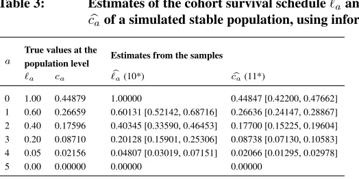
At each iteration, individuals randomly die depending on the corresponding age-specific probabilities of death. Applying (9*), (10*), and (11*), we get estimates for the survival schedule and the stable age structure for all samples. Finally, combining the results from the 100 samples, we obtain mean values and empirical confidence intervals for all the estimates and compare them with the survival schedule used in the data simulation and the age structure of the whole population. The results displayed in Table 3 show that our method to estimate`a andca for stable populations may provide serviceably accurate
results. Differences among the estimates and the true values observed at the population level are due to the randomness in the data simulation and the sampling process, and also because of the rounding to integer values of the population counts. All true values fall within the 95% empirical confidence intervals of the estimates.
Table 3: Estimates of the cohort survival schedule`ab and the age structure
b
caof a simulated stable population, using information on life left
a
True values at the
Estimates from the samples population level
`a ca `ba(10*) cba(11*)
0 1.00 0.44879 1.00000 0.44847 [0.42200, 0.47662] 1 0.60 0.26659 0.60131 [0.52142, 0.68716] 0.26636 [0.24147, 0.28867] 2 0.40 0.17596 0.40345 [0.33590, 0.46453] 0.17700 [0.15225, 0.19604] 3 0.20 0.08710 0.20128 [0.15901, 0.25306] 0.08738 [0.07130, 0.10583] 4 0.05 0.02156 0.04807 [0.03019, 0.07151] 0.02066 [0.01295, 0.02978]
5 0.00 0.00000 0.00000 0.00000
Note: Estimates from 100 samples of size 1,000 that are randomly taken from a stable population of 234,248 indi-viduals. The samples are followed until death. Values between square brackets represent 95% empirical confidence intervals.
5. The 1805 cohort life table of Swedish females
As an example of application with actual data, we aim to recover the 1805 cohort life table of Swedish females by applying Equations (9*) and (10*) to data on population counts. The goal is to create a scenario in which we simulate the ‘capture’ of the Swedish females in 1805, ignoring their ages, and follow this group of individuals until extinction. First, we ‘capture’ the population in 1805, as in a census. Next, we follow those individuals along the 19th century by recording the number of individuals still alive at each subsequent five-year period, obtaining theNea(t)values. Finally, applying (9*) we
data comes from the Human Mortality Database (2018) (henceforth HMD). The results presented below are fully reproducible from the R code (R Core Team 2018) and data available in the supplementary materials.
5.1 Estimation of the growth rate
An estimate of the stable growth rateris needed to apply the formulas in this article. This parameter can be estimated in various ways because all scalable stable population param-eters grow exponentially at the same rate, including the number of births and deaths, and population size. Keyfitz and Caswell (2005, Chapter 5.2) provide an interesting discus-sion about how to estimate the growth rate from a single census, given the assumption of a stable population in which all cohorts follow the same life table. However, their approach requires knowledge of the number of individuals at a minimum of two different ages, and the probability of surviving between them. This is not the case in a context in which the ages of the population are unknown, and the survival schedule is estimated depending on the growth rater, as shown in (2*) and (10*).
If the number of birthsB(t)at first observation can be assessed, one could simply consider
r=B(t)−D(t)
N(t) =
B(t)−De(0,t)
e
N(0,t) .
When that information is not available,rcan be estimated if the entire population (or a random sample) is observed at two time pointst1andt2so that information is available
onN(t1)andN(t2). This may be the most convenient approach in many real-world
scenarios. If that is the case,
(12) r= ln
N(t2)−lnN(t1)
t2−t1
,
a formula that follows from the definition of a stable population (Keyfitz and Caswell 2005: 12). We use (12) to estimate the growth rate of the Swedish female population in the 19thcentury, using the total populations counts of 1805 and 1895 from the HMD:
r=ln
N(1895)
−ln
N(1805)
1895−1805 = ln
2,509,076
−ln
1,249,946
1895−1805 ≈0.00774.
5.2 Reconstruction of the survival curve
of individuals from that initial population who are still alive in 1810. In terms of the available data, this corresponds to the number of Swedish females above age 5 in 1810,
N5+(1810) = Ne5(1805) = 1,105,919. We follow the same procedure to obtain
N10+(1815) = Ne10(1805) =1,007,581,N15+(1820) = Ne15(1805), and so on. All
these population counts were affected by migration flows. Nevertheless, in the stable population model, we assume closure to migration, something necessary to apply our method to estimate age-specific survival in a population with unknown ages.
Once the values Ne0(1805),. . .,Ne90(1805) are available, we can apply (9*) and
(10*) to estimate the survival schedule of the 1805 cohort of Swedish females. Figure 4 presents the results by comparing the estimated survivorship with the survival curve from the corresponding cohort life table of the HMD.
Figure 4: Observed (HMD) and estimated survival schedule of the 1805
cohort of Swedish females using Equation(10*)
age
sur
viv
orship
0 5 10 15 20 25 30 35 40 45 50 55 60 65 70 75 80 85 0.0
0.2 0.4 0.6 0.8 1.0
HMD
estimated
estimated (smoothed)
Source: Human Mortality Database (2018).
The dark line in Figure 4 refers to the HMD life table. The dashed line is the result of applying (10*) to theNae (t)values. This curve is not monotonically decreasing, which
predict(), is one of the most common methods to smooth volatile data, and it is based on implementing a nonparametric approach that fits multiple regressions in a local neigh-borhood (see example of application in the R code of the supplementary materials). The similarity between the dark and yellow curves illustrates the validity of our theoretical ap-proach to estimate age-specific survival in populations with unknown ages, but in which individuals are followed until death. Moreover, it also shows that the Swedish female population in the 19thcentury was rather stable.
6. Discussion
In this article, we have extended the concept of symmetries between life lived and left from stationary to stable populations. Equations (1*) and (9*) are a generalization to sta-ble populations of previous results by Brouard (1989), Vaupel (2009), and Villavicencio and Riffe (2016), who limited their analysis to stationary populations. The stable popu-lation model represents a less restrictive setup with more potential areas of application. Further, by using the survival curve in (2*), all the usual life table functions and statistics can be calculated, including the stable age structure.
The relationship between life lived and left may be especially relevant for the study of populations in which ages are unknown, but individuals are followed until death. In Section 4 we discuss some of the challenges of applying theoretical relationships to em-pirical data, especially due to the fact that in real-world scenarios time is not continu-ous, and some adjustments are necessary to move from a continuous to a discrete-time framework. In this regard, Equations (9*), (10*), and (11*) may be more interesting to researchers dealing with actual data. Furthermore, it is remarkable that, contrary to what usually happens, the discrete equations are simpler to derive than the continuous ones, as illustrated in Figures 2 and 3. Their validity has been demonstrated in the applications of Sections 4.2 and 5.
References
Brouard, N. (1986). Structure et dynamique des populations: La pyramide des ann´ees `a vivre, aspects nationaux et exemples r´egionaux. Espace, populations, soci´et´es4(2): 157–168.doi:10.3406/espos.1986.1120.
Brouard, N. (1989). Mouvements et mod`eles de population. Yaound´e: Institut de Formation et de Recherche D´emographiques. http://iford-cm.org/images/documents pedagogique/Mouvements-et-modeles-IFORD-1989.pdf(retrieved on June 24, 2018). Euler, L. (1970). A general investigation into the mortality and multiplication of the hu-man species [translated by N. Keyfitz and B. Keyfitz].Theoretical Population Biology 1(3): 307–314.doi:10.1016/0040-5809(70)90048-1.
Goldstein, J.R. (2009). Life lived equals life left in stationary populations.Demographic Research20(2): 3–6.doi:10.4054/DemRes.2009.20.2.
Human Mortality Database (2018). [electronic resource]. Berkeley and Rostock: University of California and Max Planck Institute for Demographic Research. http://www.mortality.org(downloaded on June 4, 2018).
Keyfitz, N. and Caswell, H. (2005). Applied mathematical demography. New York: Springer. doi:10.1007/b139042.
Kim, Y.J. and Aron, J.L. (1989). On the equality of average age and average expec-tation of remaining life in a sexpec-tationary population. SIAM Review31(1): 110–113. doi:10.1137/1031005.
Lotka, A.J. (1907). Relation between birth rates and death rates.Science26(653): 21–22. doi:10.1126/science.26.653.21-a.
Lotka, A.J. (1934).Th´eorie analytique des associations biologiques: I. Principes. Paris: Hermann.
Lotka, A.J. (1939). Th´eorie analytique des associations biologiques: II. Analyse d´emographique avec application particuli`ere `a l’esp`ece humaine. Paris: Hermann.
Lotka, A.J. (1998).Analytical theory of biological populations[translated by D.P. Smith and H. Rossert]. New York: Springer. doi:10.1007/978-1-4757-9176-1.
M¨uller, H.G., Wang, J.L., Carey, J.R., Caswell-Chen, E.P., Chen, C., Papadopoulos, N., and Yao, F. (2004). Demographic window to aging in the wild: Constructing life tables and estimating survival functions from marked individuals of unknown age.Aging Cell 3(3): 125–131.doi:10.1111/j.1474-9728.2004.00096.x.
doi:10.1016/j.tpb.2007.07.003.
Preston, S.H., Heuveline, P., and Guillot, M. (2001).Demography: Measuring and mod-eling population processes. Oxford: Blackwell.
R Core Team (2018). R: A language and environment for statistical computing. Vienna: R Foundation for Statistical Computing. http://www.r-project.org.
Riffe, T. (2015). The force of mortality by years lived is the force of increment by years left in stationary populations. Demographic Research 32(29): 827–834. doi:10.4054/DemRes.2015.32.29.
United Nations (1968). The concept of a stable population: Application to the study of populations of countries with incomplete demographic statistics. New York: United Nations, Department of Economic and Social Affairs, Population Division. http://www.un.org/en/development/desa/population/publications/manual/model/stable-population.shtml(retrieved on December 28, 2017).
Vaupel, J.W. (2009). Life lived and left: Carey’s equality.Demographic Research20(3): 7–10.doi:10.4054/DemRes.2009.20.3.