Unger

(1)

Forestry & Natural-Resource Sciences Last Correction: Sep. 19, 2014

A TEST OF THE MEAN DISTANCE METHOD FOR FOREST

REGENERATION ASSESSMENT

Daniel Unger, Jeremy Stovall, Brian Oswald, David Kulhavy, I-Kuai Hung

Stephen F Austin State University, Texas, USA

Abstract. A new distance-based estimator for forest regeneration assessment, the mean distance

method, was developed by combining ideas and techniques from the wandering quarter method, T-square sampling and the random pairs method. The performance of the mean distance method was compared to conventional 4.05 square meter plot sampling through simulation analysis on 405 square meter blocks of a field surveyed clumped distribution and a computer generated random distribution at different levels of density of 100, 50 and 25%. The mean distance method accurately estimated density on the random populations but the mean distance method estimates were more variable than those of 4.05 square meter plot sampling. The mean distance method overestimated actual density and was less precise than plot sampling when both methods were tested on the clumped populations. The optimum sample sizes needed for the mean distance method to achieve the same precision as 4.05 square meter plot sampling at all three density levels, for both the random and clumped spatial distributions, were at least 10 times larger than the sample size used for 4.05 square meter plot sampling.

Keywords: Key Words: sampling, plot, distance, accuracy, seedlings.

1 Introduction

Estimating the density of regeneration, or number of seedlings per unit area, on a given site is important to foresters for assessing existing regeneration, determin-ing reforestation needs, and determindetermin-ing if reforesta-tion efforts have been successful. A variety of sampling methods have been developed for estimating regenera-tion density. The majority of the methods fall into two general categories: plot sampling and distance sampling (Payandeh and Ek, 1986). Plot sampling is the tradi-tional approach that involves establishing fixed size plots within an area, counting the trees within each plot, and then converting the tree counts to a density estimate. On the other hand, distance sampling involves measur-ing the distance(s) from a sample point or tree to another tree(s) within an area and then using this distance(s) to estimate density. Our objective was to compare the per-formance of a new distance-based method, known as the mean distance method, as an alternative to traditional plot sampling. Both methods were evaluated through computer simulation analysis on 405 square meter blocks (0.1 acre) of a field surveyed clumped distribution and a computer generated random distribution at different density levels of 100, 50 and 25%.

2 Distance Sampling

Distance sampling has attracted the attention of re-searchers over the past 50 years as a means of estimating density. Its main attraction is that it is fast, easy to use, and one or more distances are always recorded at each sample point. In contrast, plot sampling can sometimes be a very time consuming process, boundary trees may be overlooked, and some plots may have no tallies.

Past attempts to develop a robust distance-based den-sity estimator have not been very successful. In general, distance estimators are not robust and tend to be bi-ased when the spatial distribution of the population un-der consiun-deration does not represent a spatially random distribution (Persson, 1971). The lack of robustness is of concern because plants in natural populations tend to be aggregated, not distributed randomly (Patil et al., 1979). The major weakness of density estimators is that their bias is dependent on the spatial distribution of the population (Delince, 1986). Some distance estimators have been shown to be unbiased over a wide range of spatial patterns if the estimators are adjusted accord-ing to the spatial pattern, but this adjustment would necessitate additional tests to determine a population’s spatial distribution before estimating density.

(2)

Pollard (1971) used a maximum likelihood method to estimate forest density from a random point using dis-tances between points and provides examples of using two nearest trees to a random point where the stan-dard deviation to the second tree is reduced by 30. He found that the number of sample points required to es-timate density with a prescribed accuracy does not de-pend on the density being measured and estimates of large diameter tree densities were reliable. Hanberry et al. (2011) compared the Pollard (1971) and the Morisita (1957) methods for estimation of tree density by ana-lyzing spacing methods and concluded that the Morisita estimator outperformed the Pollard estimator in non-random and clustered distribution under typical forest conditions. Although researchers have studied distance sampling in quantifying vegetation, no study to date has provided a distance based method of density esti-mation as an alternative to traditional plot sampling. This research was undertaken to reinvigorate the desire and need for a fast and efficient method of density esti-mation as an alternative to plot sampling.

This study evaluated a new distance-based density es-timator that combines the attractive features of the wan-dering quarter method (Catana, 1963), T-square sam-pling (Aherne and Diggle, 1978; Diggle, 1975; Diggle, 1977) and the random pairs method (Cottam and Curtis, 1949; Cottam and Curtis, 1955). The performance of the new distance estimator, which was evaluated through simulation analysis, was proposed as a statistically ro-bust, fast and easier estimator to implement than tradi-tional plot sampling.

3 Methods

The new method of density estimation, to be known as the mean distance method, incorporates the feature of making multiple distance measurements between trees in one general direction from the wandering quarter method (Catana 1963). Because most natural stands tend to be aggregated, directional measurement gives the estimator mobility and forces it out of clumped ar-eas into open arar-eas, or out of open arar-eas into clumped areas, depending on the location of the sample point. By sampling through a population and not remaining stationary, the estimator is better able to determine the overall average distance between trees. This overall av-erage distance is used to determine the avav-erage area oc-cupied per tree. The inverse of the average area per tree is the density estimate which was incorporated from the random pairs method for ease of calculation. The fea-ture of measuring the distance from one tree to its near-est neighbor across a 180 degree line was incorporated from T-square sampling to simplify locating seedlings in the field.

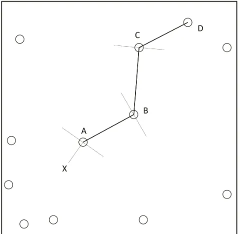
Figure 1: Procedure of the mean distance method as-sumingsequals three. The circles represent trees,X is a sample point, andAis the closest tree to sample point X. Measure lineA−B becauseBis the nearest tree to Alying beyond a line drawn throughAwhich is perpen-dicular to lineX−A; measure lineB−C becauseC is the nearest tree toB lying beyond a line drawn through Bwhich is perpendicular to lineA−B; and measure line C−D becauseD is the nearest tree toC lying beyond a line drawn through C which is perpendicular to line B−C.

The procedure (Fig. 1) for obtaining the necessary distances for the mean distance method at each sample point within a population follows:

1. Beginning with a randomly located sample point (X), locate the closest tree (A).

2. Measure the distance from the closest tree (A) to its nearest neighbor (B) lying beyond a line drawn perpendicular to the sample point-closest tree line (lineX−A) which intersects the closest tree (A).

3. Next, measure the distance from the last tree mea-sured (B) to its nearest neighbor (C) lying beyond a line drawn perpendicular to the last measured dis-tance line (lineA−B) which intersects the last tree measured to (B).

(3)

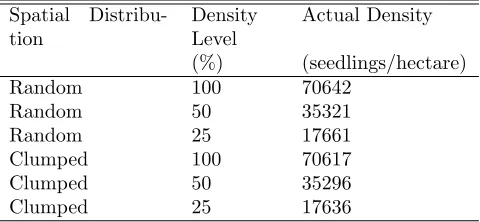
Table 1: Seedlings per hectare of the computer generated random and field surveyed clumped spatial distributions at 100, 50 and 25% of density level.

Spatial Distribu-tion Density Level Actual Density (%) (seedlings/hectare)

Random 100 70642

Random 50 35321

Random 25 17661

Clumped 100 70617

Clumped 50 35296

Clumped 25 17636

By assuming the area occupied by a tree is represented by a hexagon and that the average of the distances mea-sured represents the average distance between trees, one can apply the following formula discussed by Cottam and Curtis (1949, 1955) to estimate density at each sam-ple point:

di= 43560 0.8661(si)2

wheredi = population density estimate per acre at sam-ple point i, si = average of the distances measured at sample pointi in feet.

Density can then be estimated for the entire popula-tion by using the following formula:

D= Pn

1di n

where D = estimated population density, n = number of sample points.

The estimated variance of the population (V) is cal-culated by the following formula:

V = Pn

1(di−D) 2 (n−1)

4 Data Analysis and Results

The mean distance method was evaluated using com-puter simulation. Distances were measured to the near-est 0.254 centimeters (0.1 inch). Simulation allowed tnear-est- test-ing the mean distance method at different population densities and spatial distributions, and the determina-tion of a reasonable value ofs, the number of distances measured per sample point. The mean distance method was compared to 4.05 square meter plot sampling.

The first step of the simulation analysis involved ob-taining clumped and random seedling populations on which to conduct the density estimation. Mapped

seedling data representing a clumped distribution of 2,859 seedling locations in a 405 square meter block within a 15-month-old clearcut in central Pennsylvania were used. An artificial random seedling distribution was generated in computer with 2,860 seedling locations within a 405 square meter block, representing the same density as the field surveyed data. These two distribu-tions were further resampled to 50 and 25% population levels to represent 3 different populations representing 100, 50, and 25% of actual density to test the density estimator across variable population densities (Tab. 1). A Fortran based computer program called REGEN was written to simulate the mean distance method and the 4.05 square meter plot sampling. The program was writ-ten to allow the following parameters to be varied: (1) the density estimator, (2) the spatial pattern of regener-ation, (3) the seedling density, (4) the number of repli-cations, (5) the sample size, and (6) the number of dis-tances measured per sample point for the mean distance method. The program calculates the average density es-timate, average variance of the mean and average coeffi-cient of variation over all replications of a given sample size.

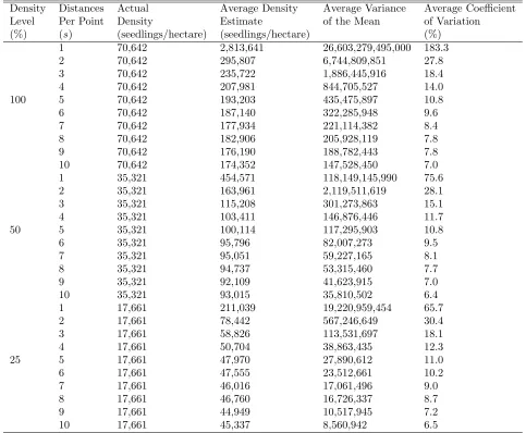
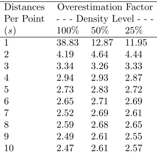
REGEN was used in initial trials of the mean distance method to determine the optimum value ofs, the num-ber of distances measured per sample point. Twenty-five replications of sample size 30, withs ranging from one to ten, were tested on three densities in the random dis-tribution (Tab. 2). The results from these initial trials were evaluated to determine the proportions that the mean distance method overestimated actual density of all three density levels of random distribution at all dis-tances tested (Tab. 3). The mean distance method’s overestimation of actual population density decreased as the number of distances measured per sample point increased, but remained approximately equal for a given density regardless of population density when the value of s was greater than one. The average variance of the mean for the mean distance method decreased as the number of distances measured per sample point in-creased, but was higher at any distance and density than the average variance of the mean for 4.05 square meter plot sampling when tested on the three densities in the random distribution with 500 replications of sample size 30 (Tab. 4). Average coefficient of variation (CV) for the 4.05 square meter plot ranged from 3 – 7%, with higher average CV’s at lower densities (Tab. 4). By con-trast, average CV’s were 10 – 11% for the mean distance method at all densities if 5 distances were measured, and as low as 6 – 7% when up to 10 distances were measured (Tab. 2).

(4)

Table 2: Average density estimate, average variance of the mean and average coefficient of variation for the mean distance method on 100, 50 and 25% density levels of the random distribution using 25 replications of sample size 30.

Density Distances Actual Average Density Average Variance Average Coefficient Level Per Point Density Estimate of the Mean of Variation (%) (s) (seedlings/hectare) (seedlings/hectare) (%)

1 70,642 2,813,641 26,603,279,495,000 183.3

2 70,642 295,807 6,744,809,851 27.8

3 70,642 235,722 1,886,445,916 18.4

4 70,642 207,981 844,705,527 14.0

100 5 70,642 193,203 435,475,897 10.8

6 70,642 187,140 322,285,948 9.6

7 70,642 177,934 221,114,382 8.4

8 70,642 182,906 205,928,119 7.8

9 70,642 176,190 188,782,443 7.8

10 70,642 174,352 147,528,450 7.0

1 35,321 454,571 118,149,145,990 75.6

2 35,321 163,961 2,119,511,619 28.1

3 35,321 115,208 301,273,863 15.1

4 35,321 103,411 146,876,446 11.7

50 5 35,321 100,114 117,295,903 10.8

6 35,321 95,796 82,007,273 9.5

7 35,321 95,051 59,227,165 8.1

8 35,321 94,737 53,315,460 7.7

9 35,321 92,109 41,623,915 7.0

10 35,321 93,015 35,810,502 6.4

1 17,661 211,039 19,220,959,454 65.7

2 17,661 78,442 567,246,649 30.4

3 17,661 58,826 113,531,697 18.1

4 17,661 50,704 38,863,435 12.3

25 5 17,661 47,970 27,890,612 11.0

6 17,661 47,555 23,512,661 10.2

7 17,661 46,016 17,061,496 9.0

8 17,661 46,760 16,726,337 8.7

9 17,661 44,949 10,517,945 7.2

10 17,661 45,337 8,560,942 6.5

determined to be the smallest value where the mean dis-tance method overestimated the actual population den-sities of all three density levels of the random distribu-tion at approximately the same propordistribu-tions. A large number of distances would render the method ineffec-tive when considering the time required to complete a sample. The optimum value of swas determined to be three.

Because the mean distance method overestimated the three random distribution densities at all values of sit was inferred that the mean distance method was un-derestimating the average distance between trees. The mean distance method was measuring less than the ac-tual distance needed, resulting in the overestimation

bias. It was determined that the average distance ob-tained between trees when s equals three represented only 55% of the average distance needed (Tab. 5).

The original program REGEN was altered by divid-ing the sample point average distance obtained between trees by 0.55, thereby increasing the average physical distance measured between trees and hence the average area occupied per tree, to adjust for the overestimation bias and provide an accurate average density estimate and to test for robustness via a new formula. The ad-justed formula is:

(5)

Table 4: Average density estimate, average variance of the mean and average coefficient of variation for 4.05 square meter plot sampling on three densities of the random distribution using 500 replications of sample size 30.

Density Actual Average Density Average Variance Average Coefficient Level Density Estimate of the Mean of Variation (%) (seedlings/hectare) (seedlings/hectare) (%)

100 70,642 70,358 5,796,740 3.4

50 35,321 35,185 2,970,126 4.9

25 17,661 17,791 1,467,529 6.8

Table 6: Average density estimate, overestimation, average variance of the mean and average coefficient of variation for the mean distance method (using the 0.55 adjustment when s equals three) on the three random distribution densities using 500 replications of sample size 30.

Distances Actual Average Density Overestimation Average Variance Average Coefficient Per Point Density Estimate of the Mean of Variation (s) (seedlings/hectare) (seedlings/hectare) (%) (%)

3 70,642 71,600 1.014 185,406,741 19.0

3 35,321 35,847 1.015 37,010,695 17.0

3 17,661 17,715 1.003 15,394,389 22.1

Table 3: Overestimation factors ([average density esti-mate – actual density]/actual density) for the mean dis-tance method on three densities of the random distribu-tion using 25 replicadistribu-tions of sample size 30.

Distances Overestimation Factor Per Point Density Level -(s) 100% 50% 25% 1 38.83 12.87 11.95 2 4.19 4.64 4.44 3 3.34 3.26 3.33 4 2.94 2.93 2.87 5 2.73 2.83 2.72 6 2.65 2.71 2.69 7 2.52 2.69 2.61 8 2.59 2.68 2.65 9 2.49 2.61 2.55 10 2.47 2.61 2.57

wheredi = population density estimate per acre at sam-ple point i, si = average of the distances measured at sample pointiin feet.

The mean distance method was then tested on the three random distribution densities with 500 replications of sample size 30 whensequals three (Tab. 6). The re-sults of the tests indicate the overestimation bias was corrected. The mean distance method’s average den-sity estimates for all three random population densities

Table 5: Expansion factors (average measured dis-tance/actual distance needed) for the mean distance method on the three random distribution densities using 25 replications of sample size 30 whensequals three.

Density Average Measured

Actual Dis-tance

Expansion

Level Distance Needed Factor

(%) (cm) (cm)

100 22.12 40.41 0.55

50 31.65 57.15 0.55

25 44.30 80.85 0.55

were within 1.5% of true population density and in close agreement with 4.05 square meter plot sampling results. The results also show that the mean distance method’s average variance of the mean when using the 0.55 ad-justment was higher than the average variance of the mean of 4.05 square meter plot sampling for an equiv-alent density, sample size and number of replications. Average CV’s were relatively high for the mean distance method, ranging from 19 – 22 % wheres= 3 (Tab. 6), as compared to 3 – 7% for the 4.05 square meter plot methodology (Tab. 4).

(6)

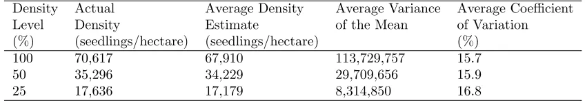
Table 7: Average density estimate, overestimation, average variance of the mean and average coefficient of variation for the mean distance method (using the 0.55 adjustment when s equals three) on the three clumped distribution densities using 500 replications of sample size 30.

Distances Actual Average Density Overestimation Average Variance Average Coefficient Per Point Density Estimate of the Mean of Variation (s) (seedlings/hectare) (seedlings/hectare) (%) (%)

3 70,617 654,535 9.269 131,109,814,367 55.3

3 35,296 646,187 18.307 4,896,588,697,138 342.4

3 17,636 44,801 2.540 396,354,779 44.4

Table 8: Average density estimate, average variance of the mean and average coefficient of variation for 4.05 square meter plot sampling on the three clumped distribution densities using 500 replications of sample size 30.

Density Actual Average Density Average Variance Average Coefficient Level Density Estimate of the Mean of Variation (%) (seedlings/hectare) (seedlings/hectare) (%)

100 70,617 67,910 113,729,757 15.7

50 35,296 34,229 29,709,656 15.9

25 17,636 17,179 8,314,850 16.8

square meters was also tested on all three clumped pop-ulation densities with 500 replications of sample size 30 (Tab. 8). The average density estimates for the mean distance method were not close to the true clumped pop-ulation densities and the average variance of the mean and average coefficient of variation for the mean distance method at all three clumped population densities when s equals three was higher than the average variance of 4.05 square meter plot sampling for an equivalent den-sity, sample size, and replication. Even 4.05 square me-ter plot sampling performed more poorly when seedlings were clumped, with average CV’s of 16 – 17% (Tab. 8) as compared with 3 – 7 % for randomly distributed seedlings (Tab. 2).

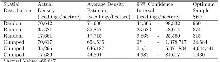
Ninety-five percent confidence intervals of density es-timate for both 4.05 square meter plot sampling and the mean distance method, plus the optimum sample size needed for the mean distance method to achieve 4.05 square meter plot sampling precision, were determined for all three density levels of the random and clumped spatial distributions (Tabs. 9-10). All confidence in-tervals of the density estimate for 4.05 square meter plot sampling were smaller than the confidence inter-vals of density estimate for the mean distance method for an equivalent density level and spatial pattern when s equals three. The sample sizes needed for the mean distance method to achieve 4.05 square meter plot sam-pling precision at any density level and spatial pattern were at least ten times larger than the sample size of 30 used by a 4.05 square meter plot.

5 Discussion

When calculating density at each sample point, the mean distance method’s average density estimates were in close agreement with the random distributions, as were the density estimates for 4.05 square meter plot sampling, but the mean distance method was more vari-able than plot sampling. The mean distance method overestimated actual density and was less precise than 4.05 square meter plot sampling when both methods were tested on the clumped distributions. Since the optimum sample sizes needed for the mean distance method to achieve the same precision as 4.05 square me-ter plot sampling at all three density levels of the random and clumped spatial distributions were at least 10 times larger than the sample size used by 4.05 square meter plot sampling, it would not be practical to implement, and would prohibit the use of the mean distance method as proposed.

(7)

Table 9: Density estimate confidence interval (95%) for 4.05 square meter plot sampling on all three densities of the clumped and random distributions using 500 replications of sample size 30.

Spatial Actual Average Density 95% Confidence Distribution Density Estimate Interval

(seedlings/hectare) (seedlings/hectare) (seedlings/hectare) Random 70,642 70,358 65,541 - 75,174 Random 35,321 35,185 31,737 - 38,631 Random 17,661 17,791 15,363 - 20,214 Clumped 70,617 67,910 46,579 - 89,239 Clumped 35,296 34,229 23,327 - 45,129 Clumped 17,636 17,179 11,411 - 22,944

Table 10: Density estimate confidence interval (95%) and optimum sample size needed to achieve 4.05 square meter plot sampling precision for the mean distance method (using the 0.55 adjustment whensequals three) on all three densities of the clumped and random distributions using 500 replications of sample size 30.

Spatial Actual Average Density 95% Confidence Optimum Distribution Density Estimate Interval Sample

(seedlings/hectare) (seedlings/hectare) (seedlings/hectare) Size

Random 70,642 71,600 44,366 - 98,832 960

Random 35,321 35,847 23,680 - 48,014 374

Random 17,661 17,715 9,868 - 25,560 315

Clumped 70,617 654,535 0* - 1,378,717 34,584 Clumped 35,296 646,187 0 # - 5,071,834 4,944,441 Clumped 17,636 44,801 4,982 - 84,617 1,430

∗_{Actual Value: -69,647}

#_{Actual Value: -3,779,461}

Since the overestimation bias can be adjusted by in-corporating an overestimation bias constant the mean method shows promise at calculating density in situa-tion such as pole size stand or larger when the average distance between trees would be greater. This would re-duce the overestimation bias and decrease the variability of the mean distance method and make it a more likely alternative to traditional milacre plot sampling.

The mean distance method was shown not to be a valid replacement for traditional milacre plot sampling for quantifying forest regeneration due to the close spac-ing of seedlspac-ings on a forest floor. However, the mean distance method did perform fairly well within a ran-dom distribution but not within a clustered or clumped population. The mean distance method may be a bet-ter choice in rangeland-shrub or dry forest communities where regeneration is less clustered or within large diam-eter tree conditions where the average distance between trees is greater.

Acknowledgements

The authors wish to express their gratitude to the peer-review process and in particular to the reviewers of this paper for their insightful comments and suggestions.

References

Aherne, W.A., and P.J. Diggle. 1978. The estimation of neuronal population density by a robust distance method. J. of Microscopy. 114:285-293.

Catana, J.A. 1963. The wandering quarter method of estimating population density. Ecology. 44:349-360.

Cottam, G., and J.T. Curtis. 1949. A method for mak-ing rapid surveys of woodlands by means of pairs of randomly selected trees. Ecology. 30:101-104.

(8)

Delince, J. 1986. Robust density estimation through dis-tance measurements. Ecology. 67:1576-1581.

Diggle, P.J. 1975. Robust density estimation using dis-tance methods. Biometrika. 62:39-48.

Diggle, P.J. 1977. A note on robust density estimation for spatial point patterns. Biometrika. 64:91-95.

Hanberry, B.B., S. Fraver, H.S. He, J. Yang, D.C. Dey and B.J. Palik. 2011. Spatial pattern corrections and sample sizes for forest density estimators of historical tree surveys. Landscape Ecol. 26:59-68.

Morisita, M. 1957. A new method for the estimation of density by the spacing method, applicable to non-randomly distributed populations. Seiri Seitai. 7:134-144.

Patil, S.A., K.P. Burnham, and J.L. Kovner. 1979. Non-parametric estimation of plant density by the distance method. Biometrics. 35:597-604.

Payandeh, B., and A.R. Ek. 1986. Distance methods and density estimators. Canadian J. of For. Res. 16:918-924.

Persson, O. 1971. The robustness of estimating den-sity by distance measurements. P. 175-187 in Statis-tical ecology: Sampling and modeling biological pop-ulations and population dynamics, Patil, G.P., E.C. Pielou, and W.E. Waters (eds.). The Pennsylvania State University Press, University Park, PA.