(DOI: 10.24874/jsscm.2018.12.01.04)
Numerical Study of Motion of a Spherical Particle in a Rotating Parabola
Using Lagrangian
H. Khalilia1, R. Jarrar2, and J. Asad2*
1 Dep. of Applied Computing - College of Sciences - P. O. Box 7 - PTUK – Tulkarm - Palestine e-mail: [email protected]
2 Dep. of Physics - College of Sciences - P. O. Box 7 – PTUK – Tulkarm - Palestine e-mail: [email protected]
e-mail: [email protected] [email protected]
* corresponding author
Abstract
In this paper, we study the motion of a spherical particle in a rotating parabola using the Lagrangian method. As the first step, we construct the Lagrangian of the system, and then we obtain the Euler-Lagrange equations (i.e. equation of motion of the system). The obtained equation of motion is a homogenous second order equation. Finally, we solve this equation numerically using the ode45 code which is based on Runge-Kutta method.
Keywords: Lagrangian, Equations of Motion, Numerical Calculation, Runge-Kutta, ode45
1. Introduction
In classical mechanics, the kinematics and dynamics of some simple systems including objects in free fall, simple harmonic motion, planetary motion, and the motion of charged particles in electromagnetic fields are investigated using either Newton's laws, or Lagrangian and Hamiltonian mechanics. Newtonian mechanics is based on vector quantities, i.e., mainly forces acting on the system, while Lagrangian and Hamiltonian Mechanics are based on a scalar quantity (i.e, kinetic and potential energies). The Lagrangian and Hamiltonian formalism play a central role in many areas such as: classical mechanics (Goldstein et al. 1980, Marion et al. 1988, Fowels et al. 2005), nonlinear systems and control theory (Murray 1997, Musielak et al. 2007). They are powerful tools that can be used to analyze the behavior of a vast class of systems, ranging from the motion of a single particle in a static potential field to complex many body systems (Goldstein et al. 1980, Marion et al. 1988, Fowels et al. 2005).
As a result of applying Lagrangian (or Hamiltonian) mechanics to physical systems, a set of differential equations called Euler-Lagrange equation (equations of motions) are obtained. In principle, these equations have to be solved analytically to describe the motion of the system. Unfortunately, in many cases the obtained differential equations cannot be solved analytically. As a result, we have to seek for numerical methods.
numerical calculations (in numerical approach) are powerful because they help scientists in solving many kinds of differential equations without seeking for their analytical solutions.
The outline of this paper is as follows. In Section 2, the physical description of the system is presented and the Lagrangian of the spherical particle in a rotating parabola is obtained. Section 3 provides numerical solutions of the derived equations of motion for different initial conditions. Finally, we close the paper by conclusion in Section 4.
2. Physical description of the model
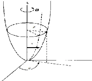
Let us consider a small spherical particle of mass (m) sliding along a surface that has a parabola
shape defined by zCs2 (Marion et al. 1988, Hatami et al. 2014), where C is constant and s is the usual cylindrical coordinate. The following assumptions are considered for the motion of the particle: the particle is in equilibrium, rotating in a circle of radius , and finally, the surface is rotating about its vertical symmetry axis with angular velocity
, as indicated in Figure 1 below (Marion et al. 1988, Hatami et al. 2014).Fig. 1. A spherical particle on a rotating parabolic surface
Below, we are going to apply the cylindrical coordinates system
s, , z
to describe the motion of the particle. Thus, the kinetic and potential energy of the particle respectively read:
1 2 2 2 2 . 2
T m s s z (1)
V mgz (2)
Our system considered here obeys the following constraints:
2
zCs (3)
t
(4)
and the derivatives of the these constraints are:
2
(6) As a result, the Lagrangian of the system can be expressed as:
1 2 4 2 2 2 2 2 2 2
L T V m s C s s s mgCs (7)
Notice here that the Lagrangian has one degree of freedom, i.e.,s. This results from the constraint equations.
Our final step in this section is obtaining the equation of motion. So, applying our Lagrangian (7)
to the following equation L d L 0
q dt q
, with qs we get the following equation of motion
(i.e. Euler-Lagrange equation)
2 2 2 2 2
4 4 0
s C ss C ss
s (8)Where we have used 2 2
2gC (Nayfeh et al. 1979).
Now, our main aim in the next sections is to obtain a numerical solution for Eq. (8) defined above.
3. Numerical solution method
One of the most celebrated methods for the numerical solution of differential equations is the one originated by Runge 1895, and elaborated by Cun 1900, Rutia 1901, Nystrom 1925 and others. There are many variants of the Runge-Kutta method, but the most widely used one is the one described below.
Given that
' , .
y f x y (9)
y x y
n n (10)
Then, one can compute in turn
,
.1
k hf x y n n
(11)
1
, .
2 2 2
k h
k hf x y
n n (12) 2 , .
3 2 2
k h
k hf x y
n n (13)
,
. 2 3k hf x h y k
n n
(14)
1
2 2 .
1 6 1 2 3 4
y y k k k k
The ode45 code is based on an explicit Runge-Kutta (4, 5) (Dormand et al. 1980). That means the numerical solver ode45 combines fourth order method and fifth order method, both of which are similar to the classical fourth order Runge-Kutta method as discussed above (Houcque et al. 2007). The modifled Runge-Kutta varies the step size, choosing the step size at each step in an attempt to achieve the desired accuracy. Therefore, the solver ode45 is suitable for a wide variety of initial value problems in practical applications. In general, ode45 is the best function to apply as a "first try" for most problems (Shampine 1994, Forsythe et al. 1977). Finally, for more details about Runge-Kutta method one can refer to Press et al. 1992. This text is written to help and teach scientists the method of numerical computing which is practical, efficient, and elegant.
Below, we propose the numerical solution for the problem (8). We consider the initial conditions as follows
0 10
s s (16)
0s s (17)
In Appendix A, we show the code we built to obtain the numerical results for Eq. (8).
4. Simulation results and discussion
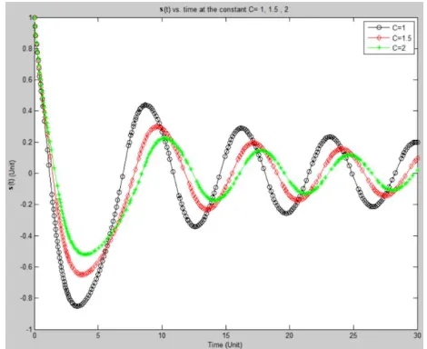
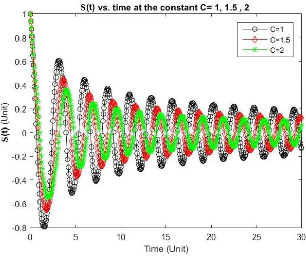
Figures 2- 5 show the radial position s t
of the particle against the time. In Figs. 2- 4, we plot
s t for three different values of (i.e., 1,1.5, 2) and for each value of we consider three values for the constant C (i.e., C1,1.5, 2). The position ( )s t of the particle looks like a damped harmonic oscillator, and this behavior is expected since the gravity pulls the particle downward and prevents it from oscillating in the same horizontal circular path. Actually, the particle moves in a spiral path with the radius s t
decreasing with time. From Figs. 2- 4 it isclear that the position s t
of the particle decreases faster as the constant C for fixed .Fig. 3. The radial position s t
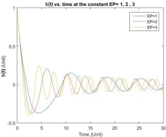
vs time for different values of the constant C, and for 2Fig. 5. The radial position s t
vs time for different values of , and for fixed value for CIn Fig. 5, we fixed Cand the position s t
is plotted against time for three different values of . It is clear from Fig. 5 that as decreases the particle needs more time to complete one rotation. Hatami et al. 2014 used a different approach to obtain numerical results for the same system considered here. The advantage of our scheme used compared to that used by Hatami et al. (2014) is that we obtained numerical results for a long time interval [0, 30] while in Hatami et al. (2014) the time interval is short [0, 10]. There are nearly good agreements between the two methods. Finally, one should keep in mind that one has to be always wary of the obtained answers, because numerical solutions are only approximations, and under certain conditions, one may get chaotic results.5. Conclusion
In this paper, ode45 code has been successfully applied in order to reach an accurate solution for the motion of a spherical particle on a rotating parabola. Radial position of the particle is depicted for the time period [0, 30]. As the main result from the present study, it is observed that the results of ode45 code are in excellent agreement with numerical ones obtained in Hatami et al. (2014), where they obtained results only for the time interval [0, 10]. So, this is the advantage point for the method used here.
References
Atkinson K, Han W, and Stewart D (2008). Numerical Solution of Ordinary Differential Equations. A John Wiley and sons, Inc., Publication
Cun K H (1900). Zeitschrift Math. Phys. 45, 23.
Dormand J R and Prince P J (1980). A family of embedded Runge-Kutta formulae. J. Comp. Appl. Math, 6:19-26.
Forsythe G, Malcolm M, and Moler C (1977). Computer Methods for Mathematical Computations. Prentice-Hall.
Fowles G R, and Cassiday G L (2005). Analytical Mechanics, 7th edn. Thomson Brooks/Cole. Goldstein H, Poole C P, and Safko J L (1980). Classical Mechanics, 3rd edn. (Addison Wesley). Hatami M, and Ganji D D (2014). Motion of a spherical particle on a rotating parabola using Lagrangian and high accuracy Multi-step Differential Transformation Method. Powder Technology 258: 94–98.
Houcque D, and Robert R (2007). Applications of MATLAB: Ordinary Differential Equations (ODE).McCormick School of Engineering and Applied Science - North western University. Marion J B, Thornton S T (1988). Classical Dynamics of Particles and Systems, 3rd edn.
(Harcourt Brace Jovanovich).
Murray R M (1997). Nonlinear control of mechanical systems: A Lagrangian perspective. Annual Reviews in Control. 21: 31- 42.
Musielak Z E, Roy D, and Swift L D (2008). Method to derive Lagrangian and Hamiltonian for a nonlinear dynamical system with variable coefficients. Chaos, Solitons and Fractals. 38(3): 894-902
Nayfeh A H, and Mook D T (1979). Nonlinear Oscillations, Willey, New York. Nystrom E I (1925). Acta Societatis Scienti aru1l1 Fcnni cac 50, No. 13, 1 to 55.
Potra F A, and Yen J (2007). Implicit Numerical Integration for Euler-Lagrange Equations via Tangent Space Parameterization. Mechanics of Structures and Machines, 19:1, 77-98. Rheinboldt W C (1995). Performance Analysis of Some Methods for Solving Euler-Lagrange
Equations. Appl. Math. Lett. Vol. 8, No. 1, pp. 77-82.
Runge C (1895). Ueber die Numerische AuftOsung von DifTercniialgleichungen, Math. Ann. 46, 167.
Rutia W (1901). Zcitschrift Math. Phys. 46,435.
Appendix A
clear al clc close all C=[1 1.5 2]; myOutput=[];
for i=1:length(C)
syms s(t) c=C(i); ep=1;
[V] = odeToVectorField( diff(s,t,2)+4*c^2*s^2*diff(s,t,2)+4*c^2*s^2*diff(s,t)+ep^2*s) M = matlabFunction(V,'vars', {'t','Y'})
figure(i)
sol = ode45(M,[0 30],[1 -1]); fplot(@(t)deval(sol,t,1), [0 30]);
xlabel('Time (Unit)') ylabel('s(t) (Unit)')
title([ 's(t) vs. time at the constant C=' num2str(c)])
h = findobj(gca,'Type','line'); x=get(h,'Xdata');
y=get(h,'Ydata');
myOutput=[myOutput [{x'},{y'}]];
end
x1 = myOutput{1}; x2 = myOutput{3}; x3 = myOutput{5}; y1 = myOutput{2}; y2 = myOutput{4}; y3 = myOutput{6}; figure
plot(x1,y1,'-ok',x2,y2,'-DR',x3,y3,'-*G') xlabel('Time (Unit)')
ylabel('s(t) (Unit)')
title('s(t) vs. time at the constant C= 1, 1.5 , 2') legend('C=1','C=1.5','C=2')
display('============ time vs. s(t) at C=1================') Result1=[x1,y1]
display('============ time vs. s(t) at C=1.5================') Result2=[x2,y2]
display('============ time vs. s(t) at C=2================')