e-ISSN: 2250-3021, p-ISSN: 2278-8719 Vol. 3, Issue 8 (August. 2013), ||V3|| PP 34-47
Use of Logarithmic Strains to Evaluate “True” Cauchy Stresses in
Finite Deformation Problems
A. E. Mohmed
1, N. M. Akasha
2And F. M. Adam
31
Dept. of Civil Engineering, Sudan University of Science and Technology, Sudan. 2
Dept. of Civil Engineering, Sudan University of Science and Technology, Sudan. 3
Dept. of Civil Engineering, Jazan University, Kingdom of Saudi Arabia.
ABSTRACT: In this paper, a Total Lagrangian formulation based on the Logarithmic strains is developed. The variation in these strains is based on the variation of the Engineering strains and the variation of Green strains. The “true” Cauchy stresses thus obtained are compared with the Engineering stresses based on the Engineering strains obtained from a Total Lagrangian formulation. The Cauchy stresses obtained based on the assumption of small Engineering shear strains are also compared with the above mentioned stresses. A Geometric nonlinear Total Lagrangian formulation applied on two-dimensional elasticity using 4-node plane finite elements was used. The formulation was implemented into the finite element program (NUSAP). The solution of nonlinear equations was obtained by the Newton-Raphson method. The program was applied to obtain stresses for three numerical examples. The evaluation of the accuracy of the formulation was based on comparing the stresses obtained with those from the other two formulations as stated above. The paper concludes that all three Total Lagrangian formulations converge to the correct solution, as expected, for small strains. For moderate and large strains, there is a clear difference between the Cauchy and the Engineering stresses. The formulation based on the Logarithmic strains results in the accurate evaluation of the “true” Cauchy stresses. These stresses can be used in the geometric and material nonlinear analyses of large deformation problems using constitutive equations based on Logarithmic strains.
Keywords: Geometric Nonlinear, Lagrangian, Large strain, Engineering stress, Cauchy stress
I. INTRODUCTION
The nonlinear behavior of almost all structures prior to reaching their limit of resistance and the use of light “tall” structures, coupled with advance in solution methods and computing facilities, have lead to the intensive use of geometric nonlinear analysis. As stated by Yang and Kuo [1] one of the main factors that have to be considered in nonlinear analysis is the calculation of internal forces. Hence, the major problem in geometrically nonlinear (GNL) finite element analysis is the need to define reference coordinates and to specify the relevant stress and strain measures. As had been shown by Ji, Waas and Bazant [2], the use of non-conjugate stress and strain increments in finite element programs can cause errors as large as 100%.
The two main finite element formulations for GNL problems are the Eulerian formulation (EFM) and the Lagrangian formulation (LFM). As stated, among others, by Yang and Kuo[1], Crisfield[3], and Zeinkiewicz and Taylor[4] LFM, in contrast to EFM, is suitable in solid mechanics applications. This is mainly due to the ease with which it handles complicated boundaries and its ability to follow material points enabling the accurate treatment of history dependent materials. There are two main approaches to LFM, namely the Total Lagrangian (TL) and the Updated Lagrangian (UL). As pointed out by Surana and Sorem[5] and Djermane et al[6] the TL formulation is recognized as the most realistic civil engineering approach. But, the main serious drawback of the TL approach, based on the Green strains, is that these strains are unsuitable for work with large strains and the 2ndPiola-Kirchhoff stresses, which are work conjugate to the Green strains, are defined in the deformed configuration and should be transformed to the un-deformed configuration. Therefore, this TL approach will result in stresses with no physical significance [3]. This is why the UL formulation is considered, by researchers ([1], [3], [4], Belytschko[7], Marinkowic et al[8] and Bonet and Wood[9]), to be the most efficient formulation and to result in the evaluation of “true” stresses. As an alternative to the use of Green strains, the LFM can be based on using the Engineering strains with the Engineering stresses and the Logarithmic strains with the Cauchy “true” stresses as work conjugate in the virtual work expression.
Logarithmic strains. Yegneh [14], introduced a constitutive model for rigid-plastic hardening materials based on the Logarithmic strain tensor. Ulz [15], presented a model of rate independent and rate dependent thermo-plasticity in the Logarithmic Lagrangian strain space at finite strains. Naghdabadi et al [16], introduced a finite deformation constitutive model for rigid plastic hardening materials based on the logarithmic strain tensor. Miehe et al [17], outlined a constitutive model and experimental results of rate dependent finite elastic-plastic behavior of polymers. Their proposed formulation was constructed in the Logarithmic strain space. Dvortein et al [18], used the Logarithmic strain measure to develop a quadrilateral finite element formulation for modeling finite strain elasto-plastic deformation processes. Hence, a formulation that enables the accurate evaluation of the true Cauchy stresses for finite deformation will be of great benefit for both geometric and material nonlinear finite element analyses.
Akasha and Mohamed [19], developed a TL formulation for the evaluation of the Cauchy stresses based on the Logarithmic strains. The formulation was based on the variation of the Engineering strains. The only limitation of the formulation was the assumption that the
Engineering shear strains are small. In a recent paper Mohamed, Akasha and Adam [20], developed a TL formulation based on the Engineering strains using the actual shear strains.
This paper presents a TL formulation for finite strain geometric nonlinear plane stress/strain problems. The formulation uses the Logarithmic strains and the true Cauchy stresses. The formulation is based on the variation of actual Engineering strains. The results for the Cauchy stresses obtained from the developed formulation are compared with the actual Engineering stresses (Ref. [20]) and the Cauchy stresses presented in Ref. [19].
II. GEOMETRICALLYNON-LINEARFINITEELEMENTTLFORMULATION
BASEDONLOGARITHMICSTRAINS
Direct proportionality between the 2ndPiola-Kirchhoff stresses, s0, and the Green-Lagrange strains, e0,
is assumed when writing the virtual work expression. In two dimensions, with reference to the initial configuration (t=0), the Green strains are given by:
𝒆𝟎 = 𝑒𝑥,𝑒𝒚,𝑒𝑥𝑦
𝑇
= 1
2 𝐅
T𝐅 − 𝐈 (1)
where F is the displacement gradient matrix
In a finite element formulation equation (1) is written as:
𝒆𝟎 = 𝒆0𝟎+ 𝒆0𝑳 = 𝐁𝟎𝒂𝟎+
1
2𝐁𝑳 𝒂𝟎 𝒂0 (2
)
where 𝒂𝟎 is the vector of nodal variables. The nonlinear strain 𝒆𝟎𝑳can be written as:
𝒆𝟎𝑳 =
1
2𝐁𝑳 𝒂𝟎 𝒂0 =
1
2𝑨𝜃𝜽0 (3)
where𝜽0= 𝜕𝑢
𝜕𝑥 𝜕𝑣
𝜕𝑥 𝜕𝑢
𝜕𝑦 𝜕𝑣
𝜕𝑦 𝑇
= 𝑮0𝒂0 (4)
u and v being the displacement components in the x and y directions respectively. Hence, the strain displacement matrix B is given from the variation in strain by:
𝑩 = 𝝏 𝒆𝟎
𝝏𝒂0 = 𝐁𝟎 + 𝐁𝑳 𝒂𝟎 = 𝑩0+ 𝑨𝜃𝑮0 (5)
In two dimensions the Engineering strains, unit stretch,𝐸𝑥and 𝐸𝑦 are defined by the change in length
per unit initial length of line elements originally oriented parallel to the x and y axes respectively. The shear strain 𝛾𝑥𝑦 is the actual angle change.
The Engineering strains, as defined above, are given in terms of Green strains by:
𝐸𝑥 = 𝑔𝑥. 𝑔𝑥 − 1 = 1 + 2𝑒𝑥− 1, 𝐸𝑦 = 𝑔𝑦. 𝑔𝑦− 1 = 1 + 2𝑒𝑦− 1 (6)
and the shear strain is defined from:
𝑒𝑥𝑦 = 𝑔𝑥. 𝑔𝑦 = 1 + 2𝑒𝑥 1 + 2𝑒𝑦 sin 𝐸𝑥𝑦
as: 𝐸𝑥𝑦 = sin−1
𝑒𝑥𝑦
1+2𝑒𝑥 1+2𝑒𝑦 (7)
where 𝑔𝑥 = 𝜕𝑅 𝜕𝑥 , 𝑔𝑦=
𝜕𝑅
𝜕𝑦 are the displacement gradient vectors, and R is the position vector after deformation.
The variation in the Engineering strains is given in terms of the variation in Green strains by:
𝛿𝑬0= 𝛿𝐸𝑥 𝛿𝐸𝑦 𝛿𝐸𝑥𝑦
𝑻
= 𝑯𝛿𝒆0 (8)
From which, the variations in the Engineering strains are given by:
𝛿𝑬0 = 𝑯𝑩𝛿𝒂0 = 𝑩∗ 𝛿𝒂0 (9)
H =
𝟏
𝒍𝒙 0 0
0 𝟏
𝒍𝒚 0
−𝒆𝒙𝒚
𝒍𝒙∗ 𝒍𝒆
−𝒆𝒙𝒚
𝒍𝒚∗ 𝒍𝒆
𝟏
𝒍𝒆
(10)
In which:
𝑙𝑥= 1 + 2 𝑒𝑥, 𝑙𝑦 = 1 + 2 𝑒𝑦, 𝑙𝑒 = 1 + 2𝑒𝑥 1 + 𝑒𝑦 − 𝑒𝑥𝑦2 (11)
The “true” Cauchy stresses are defined as the internal forces per unit area acting along the normal and two tangential directions of the deformed configuration. The Logarithmic strain ε is the strain associated with the Cauchy stress τ. In two dimensions the Logarithmic strains are defined in terms of the Engineering strains as:
𝜀𝑥= ln 1 + 𝐸𝑥 , 𝜀𝑦= ln 1 + 𝐸𝑦 , 𝜀𝑥𝑦 = 𝐸𝑥𝑦 (12)
Wherein the true shear strain is defined as the actual change in the angle (in radians) between two material line elements initially perpendicular to each other.
And the Cauchy stresses are given by:
𝝉= { 𝜏𝑥𝜏𝑦𝜏𝑥𝑦}𝑇= 𝑫 𝜺 (13)
From (12), the variation in Logarithmic strains is defined in terms of the variation in Engineering strains as:
𝛿𝜺0= 𝑳 𝛿𝑬0 = 𝑳𝑯𝑩𝛿𝒂0 = 𝑩′ 𝛿𝒂0 (14)
In which L is given by:
L =
1
1+𝐸𝑥 0 0
0 1
1+𝐸𝑦 0
0 0 1
(15)
The incremental equilibrium equations in terms of Cauchy stresses are:
−𝝋 = 𝐑 − 𝑩𝑇𝑯𝑇𝑳𝑇𝝉 𝑑𝑉
0 𝑉0
= 𝐑 − 𝑩′𝑇𝝉 𝑑𝑉
0 𝑉0
(16)
And their variation gives:
𝛿𝝋 = 𝑲𝑇∗ 𝛿𝒂0 (17)
In which the tangent stiffness matrix 𝑲𝑇 is given by:
𝑲𝑇 = 𝑲0 + 𝑲𝐿 + 𝑲𝜎 + 𝑲𝜎∗ + 𝑲𝜎∗∗ (18)
where:
𝑲0 + 𝑲𝐿 = 𝑩𝑇𝑯𝑇𝑳𝑇𝑫𝑳𝑯𝑩 𝑑𝑉0
𝑉0
= 𝑩′𝑇𝑫𝑩′𝑑𝑉
0 𝑉0
(19)
and 𝑲𝜎 is the initial stress stiffness matrix dependent on the Cauchy stress, and can be written as:
𝑲𝜎 = 𝑮0𝑇𝑷𝟎𝒊𝑮0𝑑𝑉0
𝑉0
(20)
where 𝑮0 is the matrix containing shape function derivatives (equation (4)).
and the initial stress matrix 𝑷𝟎𝒊 is defined as:
𝑷𝟎𝒊 =
𝜏𝒙∗ 𝐼 𝜏𝒙𝒚∗ 𝐼
𝜏𝒙𝒚∗ 𝐼 𝜏𝒚∗ 𝐼
(21)
where 𝐼 is 22 unit matrix. and 𝝉∗is the stress vector given by:
𝝉∗ =
𝜏𝒙∗
𝜏𝒚∗
𝜏𝒙𝒚∗
= 𝑯𝑇𝑳𝑇
𝜏𝒙
𝜏𝒚
𝜏𝒙𝒚
(22)
And the 1st additional initial stress stiffness matrix 𝑲𝜎∗ takes the following form:
𝑲𝜎∗ = 𝑩𝑇𝑷𝟎𝒊∗ 𝑩 𝑑𝑉0
𝑉0
(23)
Where 𝑷𝟎𝒊∗ the 2nd initial stress matrix is obtained from:
𝛿𝑯𝑇𝑳𝑇𝝉 = 𝑷
𝟎𝒊 ∗ 𝛿𝜺
0 = 𝑷𝟎𝒊∗ 𝑩𝛿𝒂0 (24)
𝑷𝟎𝒊∗ =
−𝜏𝑥′
𝑙𝑥
3 +
2𝑒𝑥𝑦𝜏𝑥𝑦′
𝑙𝑥2∗ 𝑙𝑒
+𝑙𝑦𝑒𝑥𝑦𝜏𝑥𝑦
′
𝑙𝑥∗ 𝑙𝑒
3
𝑒𝑥𝑦 ∗ 𝜏𝑥𝑦′
𝑙𝑒
3
−𝑙𝑦𝑒𝑥𝑦𝜏𝑥𝑦′
𝑙𝑒
3
𝑒𝑥𝑦 ∗ 𝜏𝑥𝑦′
𝑙𝑒
3
−𝜏𝑦′
𝑙𝑦
3 +
2𝑒𝑥𝑦𝜏𝑥𝑦′
𝑙𝑦2∗ 𝑙𝑒
+𝑙𝑥𝑒𝑥𝑦𝜏𝑥𝑦
′
𝑙𝑦 ∗ 𝑙3 𝑒
−𝑙𝑥𝑒𝑥𝑦𝜏𝑥𝑦′
𝑙𝑒
3
−𝑙𝑦𝑒𝑥𝑦𝜏𝑥𝑦′
𝑙𝑒
3
−𝑙𝑥𝑒𝑥𝑦𝜏𝑥𝑦′
𝑙𝑒
3
𝑒𝑥𝑦𝜏𝑥𝑦′
𝑙𝑒
3
(25)
And 𝝉′is the stress vector given by:
𝝉′ =
𝜏𝒙′
𝜏𝒚′
𝜏𝒙𝒚′
= 𝑳𝑇
𝜏𝒙
𝜏𝒚
𝜏𝒙𝒚
(26)
The 2nd additional initial stress stiffness matrix 𝑲𝜎∗∗ is of the following form:
𝑲𝜎∗∗ = 𝑩𝑉0 𝑇𝑯𝑇𝑷𝟎𝒊∗∗𝑯𝑩 𝑑𝑉0
= 𝑩∗𝑇𝑷
𝟎𝒊 ∗∗𝑩∗𝑑𝑉
0 𝑉0
(27)
Where 𝑷𝟎𝒊∗∗the 3rd initial stress matrix is obtained from:
𝛿𝑳𝑇𝝉 = 𝑷
𝟎𝒊 ∗∗𝛿𝑬
0 = 𝑷𝟎𝒊∗∗𝑯 𝑩𝛿𝒂0 (28)
and is given by:
𝑷𝟎𝒊∗∗=
−𝜏𝑥
(1 + 𝐸𝑥)2
0 0
0 −𝜏𝑦
(1 + 𝐸𝑦)2
0
0 0 0
(29)
Upon solving the incremental equilibrium equations for the displacement increments ∆𝒂0𝑖 the total
displacements 𝒂0𝑖+1 are obtained as:
𝒂0𝑖+1 = 𝒂0𝑖 + ∆𝒂0𝑖 (30)
Then, the strain increments are given by:
∆𝜺0𝑖 = 𝑳 𝑯 𝐁𝟎+ 𝐁𝑳 𝒂0𝑖+1 +
1
2𝐁𝑳 ∆𝒂0
𝑖 ∆𝒂
0
𝑖 (31)
The stress increments are then given by:
∆𝝉0𝑖 = 𝑫∆𝜺0𝑖 (32)
And the total stresses are:
𝝉0𝑖+1 = 𝝉0𝑖 + ∆𝝉0𝑖 (33)
The residual forces, for a new displacement increment, are then equal to:
−𝝋𝒊+𝟏 = 𝐑 − 𝑩𝑇𝑯𝑇𝑳𝑇𝝉
𝟎 𝒊+𝟏𝑑𝑉
0 𝑉0
= 𝐑 − 𝑩′𝑇𝝉
𝟎 𝒊+𝟏𝑑𝑉
0 𝑉0
(34)
III. NUMERICALRESULTSANDDISCUSSION
The finite element TL formulation described in the above section was implemented in the FORTRAN based program NUSAP. Three numerical examples of large deformation problems were examined to demonstrate the degree of accuracy that can be obtained by using the geometrically non-linear formulation based on 4-node isoparametric plane stress/strain elements. The results of the true Cauchy stresses obtained from the formulation based on the Logarithmic strains (Log ) are compared with Cauchy stresses obtained using the formulation presented in reference [19] (Log Re19) and the Engineering stresses from reference [20] (Eng).
3.1 Cantilever under point load at free end
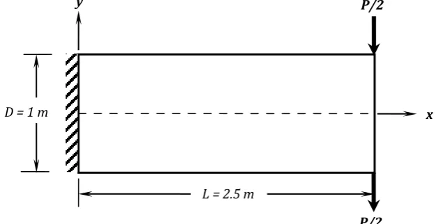
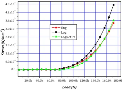
At mid-span the x-direction stress values closely agree for small and medium deformations. For large deformation there is a clear difference between the stress values with a maximum of 35.5% between the Log and Log R19 and 31% between the Log and Eng formulations. The y-direction stress values vary similarly with a maximum difference of 24% for the Log and the Log R19 and 29% for the Log and Eng formulations. For small strain, the shear stress values are in close agreement for all formulations. The Log and the Log R19 shear values closely agree up to the 140 kN load (4% maximum difference). The maximum difference between the Log and Eng shear values is about 21% for the 140 kN load. For larger loads there are marked differences between the shear values for all formulations.
At the support the x-direction stress values for the Log and Eng formulations closely agree for all loads with a maximum difference of 2%. The Log R19 values vary slightly from the Log values for large loads with a maximum difference of 7%. The y-direction stresses are in close for the three formulations for all loads. There are marked differences in the shear stress values at the support for large loads. The maximum difference is about 17.5% between the Log and the Eng values and 36% between the Log and the Log R19 values.
The differences between the Log and Log R19 values are mainly due to the assumption of small engineering shear strains in the Log R19 formulation. The differences between the Log and Eng values may be attributed to the large strain value at mid-span.
Figure (1) Cantilever plate with vertical load at free end
Table (1): Average Nodal Stress in x-direction at mid span LOAD
(N)
Stress (N/mm2) LOAD
(N)
Stress (N/mm2)
Log Log Ref19 Eng Log Log Ref19 Eng
0 0 0 0 92000 -5.61E+06 -6.63E+06 -4.86E+06
4000 -2.99E+05 -2.99E+05 -2.99E+05 100000 -5.26E+06 -6.65E+06 -4.51E+06 20000 -1.50E+06 -1.51E+06 -1.49E+06 116000 -3.22E+06 -5.70E+06 -2.82E+06 36000 -2.75E+06 -2.80E+06 -2.66E+06 132000 1.37E+06 -2.79E+06 6.57E+05 52000 -3.99E+06 -4.14E+06 -3.75E+06 148000 9.56E+06 2.94E+06 6.54E+06 68000 -5.06E+06 -5.41E+06 -4.59E+06 164000 2.24E+07 1.24E+07 1.55E+07 84000 -5.64E+06 -6.38E+06 -4.95E+06 180000 4.08E+07 2.63E+07 2.81E+07
L = 2.5 m
y P/2
x
D = 1 m
Figure (2): Average Nodal Stress in Figure (3): Average Nodal Stress in x-direction at mid span y-direction at mid span
Table (2): Average Nodal Stress in y-direction at mid span LOAD
(N)
Stress (N/mm2) LOAD
(N)
Stress (N/mm2)
Log Log Ref19 Eng Log Log Ref19 Eng
0 0 0 0 92000 2.05E+06 1.01E+06 1.99E+06
4000 2.43E+04 2.44E+04 2.43E+04 100000 3.31E+06 1.90E+06 3.02E+06 20000 1.30E+05 1.38E+05 1.20E+05 116000 7.28E+06 4.82E+06 6.08E+06 36000 2.28E+05 2.77E+05 1.77E+05 132000 1.39E+07 9.81E+06 1.09E+07 52000 2.10E+05 3.65E+05 9.64E+04 148000 2.39E+07 1.76E+07 1.80E+07 68000 1.35E+05 2.34E+05 2.89E+05 164000 3.84E+07 2.88E+07 2.79E+07 84000 1.15E+06 3.91E+05 1.22E+06 180000 5.79E+07 4.42E+07 4.11E+07
Table (3): Average Shear Stress at mid span LOAD
(N)
Stress (N/mm2) LOAD
(N)
Stress (N/mm2)
Log Log Ref19 Eng Log Log Ref19 Eng
0 0 0 0 92000 -1.08E+06 -9.87E+05 -9.32E+05
4000 -2.18E+04 -2.17E+04 -2.17E+04 100000 -1.33E+06 -1.22E+06 -1.12E+06 20000 -1.11E+05 -1.10E+05 -1.11E+05 116000 -1.95E+06 -1.83E+06 -1.54E+06 36000 -2.13E+05 -2.06E+05 -2.12E+05 132000 -2.56E+06 -2.53E+06 -1.98E+06 52000 -3.48E+05 -3.29E+05 -3.40E+05 148000 -2.75E+06 -3.08E+06 -2.25E+06 68000 -5.50E+05 -5.10E+05 -5.18E+05 164000 -1.71E+06 -2.90E+06 -2.06E+06 84000 -8.65E+05 -7.92E+05 -7.71E+05
Figure (4) Average shear stress at mid span Figure (5) Average Nodal Stress in x- direction at support 20.0k 40.0k 60.0k 80.0k 100.0k 120.0k 140.0k 160.0k 180.0k
-1.0x10⁷
-5.0x10⁶
0.0 5.0x10⁶
1.0x10⁷
1.5x10⁷
2.0x10⁷
2.5x10⁷
3.0x10⁷
3.5x10⁷
LogRef19 Eng Log
St
re
ss
(
N
/mm
2)
Load (N)
20.0k 40.0k 60.0k 80.0k 100.0k 120.0k 140.0k 160.0k 180.0k 0.0
6.0x10⁶
1.2x10⁷
1.8x10⁷
2.4x10⁷
3.0x10⁷
3.6x10⁷
4.2x10⁷
4.8x10⁷
Eng Log LogRef19
Stre
ss
(
N/m
m
2)
Load (N)
0.0 20.0k 40.0k 60.0k 80.0k 100.0k 120.0k 140.0k 160.0k 180.0k 0.0
-5.0x10⁵
-1.0x10⁶
-1.5x10⁶
-2.0x10⁶
-2.5x10⁶
-3.0x10⁶
-3.5x10⁶
Log LogRef19 Eng
Stre
ss
(
N/m
m
2)
Load (N)
0.0 20.0k 40.0k 60.0k 80.0k 100.0k 120.0k 140.0k 160.0k 180.0k 0
1x10⁷
2x10⁷
3x10⁷
4x10⁷
5x10⁷
6x10⁷
Eng LogRef19 Log
Stre
ss
(
N/m
m
2)
Figure (6) Average Nodal Stress in Figure (7) Average shear stress at Support y-direction at support
3.2 Cantilever under pure bending at free end:
A cantilever subjected to pure moment is considered. The cantilever is of dimensions L = 3000mm, D
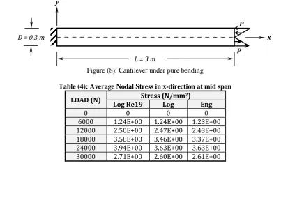
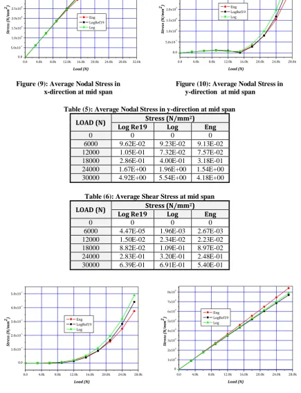
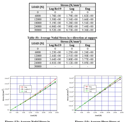
= 300 mm and thickness t = 60 mm as shown in Figure (8). The numerical values of material property parameters are Young's modulus, E = 210 GPa, and Poisson’s ratio, υ = 0.3. The structure is modeled with a mesh of 40-isoparametric elements. The mesh is of equal size elements of 150x150mm. The variations in the stresses at the support and at mid-span with load increments as computed by Log formulation are compared with the Eng formulation results from Ref [20] and the Log Re19 formulation result presented in Ref [19]. The results are presented in Figures (9) to (14) and tables (4) to (9).
As can be seen from the tables the values of the stresses are generally small. The stresses in the x-direction are in close agreement for all formulations up to the 18000N load with a difference of about 3%. The Log and Eng values clearly agree for all loads. The stresses in the y-direction and the shear stresses at mid-span are small and show a similar trend. The stresses at the support vary almost linearly and are all in close agreement for all loads. This is mainly due to the small strain values at the support.
Figure (8): Cantilever under pure bending
Table (4): Average Nodal Stress in x-direction at mid span Stress (N/mm2)
LOAD (N)
Eng Log
Log Re19
0 0
0 0
1.23E+00 1.24E+00
1.24E+00 6000
2.43E+00 2.47E+00
2.50E+00 12000
3.37E+00 3.46E+00
3.58E+00 18000
3.63E+00 3.63E+00
3.94E+00 24000
2.61E+00 2.60E+00
2.71E+00 30000
0.0 20.0k 40.0k 60.0k 80.0k 100.0k 120.0k 140.0k 160.0k 180.0k 0.0
2.0x10⁶
4.0x10⁶
6.0x10⁶
8.0x10⁶
1.0x10⁷
1.2x10⁷
1.4x10⁷
1.6x10⁷
1.8x10⁷
2.0x10⁷
2.2x10⁷
Eng LogRef19 Log
Stre
ss
(
N/m
m
2)
Load (N)
0.0 20.0k 40.0k 60.0k 80.0k 100.0k 120.0k 140.0k 160.0k 180.0k 0.0
5.0x10⁶
1.0x10⁷
1.5x10⁷
2.0x10⁷
2.5x10⁷
3.0x10⁷
3.5x10⁷ 4.0x10⁷
Eng LogRef19 Log
Stre
ss
(
N/m
m
2)
Load (N)
L = 3 m
P
P
x y
Figure (9): Average Nodal Stress in Figure (10): Average Nodal Stress in x-direction at mid span y-direction at mid span
Table (5): Average Nodal Stress in y-direction at mid span Stress (N/mm2)
LOAD (N) Eng Log Log Re19 0 0 0 0 9.13E-02 9.23E-02 9.62E-02 6000 7.57E-02 7.32E-02 1.05E-01 12000 3.18E-01 4.00E-01 2.86E-01 18000 1.54E+00 1.96E+00 1.67E+00 24000 4.18E+00 5.54E+00 4.92E+00 30000
Table (6): Average Shear Stress at mid span Stress (N/mm2)
LOAD (N) Eng Log Log Re19 0 0 0 0 2.67E-03 1.96E-03 4.47E-05 6000 2.23E-02 2.34E-02 1.50E-02 12000 8.97E-02 1.09E-01 8.82E-02 18000 2.48E-01 3.20E-01 2.83E-01 24000 5.40E-01 6.91E-01 6.39E-01 30000
Figure (11) Average shear stress at mid-span Figure (12) Average Nodal Stress in x-direction at support
Table (7): Average Nodal Stress in x-direction at support 0.0 4.0k 8.0k 12.0k 16.0k 20.0k 24.0k 28.0k 32.0k
0.0 5.0x10⁻¹ 1.0x100 1.5x100 2.0x100 2.5x100 3.0x100 3.5x100 4.0x100 Eng LogRef19 Log Stre ss ( N/m m 2) Load (N)
0.0 4.0k 8.0k 12.0k 16.0k 20.0k 24.0k 28.0k 0.0 5.0x10⁻¹ 1.0x100 1.5x100 2.0x100 2.5x100 3.0x100 3.5x100 Eng LogRef19 Log Stre ss ( N/m m 2) Load (N)
0.0 4.0k 8.0k 12.0k 16.0k 20.0k 24.0k 28.0k 0.0 1.0x10⁻¹ 2.0x10⁻¹ 3.0x10⁻¹ 4.0x10⁻¹ 5.0x10⁻¹ Eng LogRef19 Log Stre ss ( N/m m 2) Load (N)
Stress (N/mm2) LOAD (N) Eng Log Log Re19 0 0 0 0 1.82E+00 1.79E+00 1.78E+00 6000 3.66E+00 3.54E+00 3.50E+00 12000 5.54E+00 5.28E+00 5.19E+00 18000 7.44E+00 7.00E+00 6.86E+00 24000 9.36E+00 8.73E+00 8.52E+00 30000
Table (8): Average Nodal Stress in y-direction at support Stress (N/mm2)
LOAD (N) Eng Log Log Re19 0 0 0 0 1.24E+00 1.25E+00 1.23E+00 6000 2.50E+00 2.51E+00 2.44E+00 12000 3.77E+00 3.80E+00 3.64E+00 18000 5.05E+00 5.12E+00 4.81E+00 24000 - - - 30000
Figure (13): Average Nodal Stress in Figure (14): Average Shear Stress at y-direction at support support
Table (9): Average Shear Stress at support Stress (N/mm2)
LOAD (N) Eng Log Log Re19 0 0 0 0 1.24E+00 1.25E+00 1.23E+00 6000 2.50E+00 2.51E+00 2.44E+00 12000 3.77E+00 3.80E+00 3.64E+00 18000 5.05E+00 5.12E+00 4.81E+00 24000 6.36E+00 6.46E+00 5.97E+00 30000
3.3 Clamped beam under point force
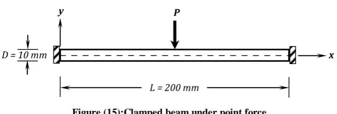
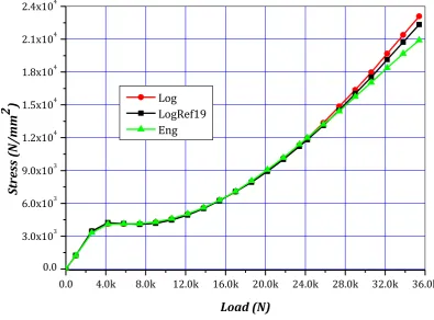
A beam with two-fixed ends is considered. The beam is of length L = 200mm, height D = 10mm and thickness 1 mm as shown in Figure (15). The numerical values for material property parameters are Young's modulus, E = 210 GPa, Poisson's ratio, υ = 0.3. The beam is modeled with a mesh of 20-elementes.
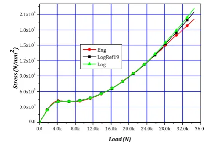
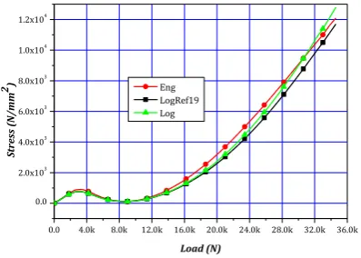
The variation of the stresses at the support and at mid-span with the load increments as computed from the Log formulation are compared with the Eng formulation results (Ref.[20]), and the Log Re19 formulation results(Ref.[19]) in Figures (16) to (21).
0.0 4.0k 8.0k 12.0k 16.0k 20.0k 24.0k 28.0k 0.0 5.0x10⁻¹ 1.0x100 1.5x100 2.0x100 2.5x100 3.0x100 Eng LogRef19 Log Stre ss ( N/m m 2) Load (N)
Figure (15):Clamped beam under point force
Tables (10), (11) and (12) show the values for average nodal stresses at mid-span. Very large loads were applied in this example resulting in large strains.
The Log values are the closest to the LogRe19 values for direct stresses at the support. A similar trend is shown by the values of the stresses in the x-direction at mid span with a maximum percentage difference between the Log and Log Re19 values of about 3% (around 10% for Eng). The stress at mid-span in the y-direction shows a similar variation with the three stress values in close agreement and continuously increasing. The maximum difference between the Log values and Eng values is around 7% and that between the Log values and the Log R19 values is 9%. The Eng shear stress at mid-span values are large, compared to the values for Log Re19 and for Log, and all three formulations show almost a linear variation. The Log Re19 shear values differ from the Eng values by about 104% as a result of the large strains and the assumption that the Engineering shear strain is small in the Log R19 formulation. The maximum difference between the Log shear values and Log R19 values is 32% as a result of this assumption. Thus, the assumption that the shear strain is small limits the use of the Log Re19 formulation for cases of small shear strain. The maximum difference of 38% between the shear values of the Log and Eng formulations is mainly due to the effect of large strains. Table (13) and Figure (22) show the maximum principal stresses at mid-span for the three formulations. These are almost identical for small and medium strain values with a maximum difference of about 3% between the Log and the Log R19 values. The maximum difference between the Log and Eng values is 9.5%. Hence, the stresses obtained using the Log formulation are considered to be an accurate measure of the true Cauchy stresses in large strain GNL.
Figure (16): Average Nodal Stress in Figure (17): Average Nodal Stress in x-direction at support y-direction at support 0.0 4.0k 8.0k 12.0k 16.0k 20.0k 24.0k 28.0k 32.0k 36.0k
0 1x10³
2x10³
3x10³
4x10³
5x10³
6x10³
7x10³
8x10³
9x10³
Eng LogRef19 Log
Stre
ss
(
N/m
m
2)
Load (N)
0.0 4.0k 8.0k 12.0k 16.0k 20.0k 24.0k 28.0k 32.0k 36.0k 0.0
3.0x10²
6.0x10²
9.0x10²
1.2x10³
1.5x10³
1.8x10³
2.1x10³
2.4x10³
2.7x10³
3.0x10³
Eng LogRef19 Log
Stre
ss
(
N/m
m
2)
Load (N) L = 200 mm
y P
x
Figure (18): Average Shear Stress Figure (19): Average Nodal Stress in at support x-direction at mid-span
Table (10): Average Nodal Stress in x-direction at mid span LOAD
(N)
Stress (N/mm2) LOAD
(N)
Stress (N/mm2)
Log Ref19 Log Eng Log Ref19 Log Eng
0 0 0 0 17800 7.47E+03 7.48E+03 7.52E+03
1000 1.23E+03 1.25E+03 1.23E+03 19400 8.40E+03 8.43E+03 8.50E+03 2600 3.32E+03 3.46E+03 3.31E+03 21000 9.44E+03 9.50E+03 9.55E+03 4200 4.10E+03 4.23E+03 4.10E+03 22600 1.06E+04 1.07E+04 1.07E+04 5800 4.12E+03 4.15E+03 4.13E+03 24200 1.18E+04 1.19E+04 1.19E+04 7400 4.12E+03 4.07E+03 4.14E+03 25800 1.31E+04 1.33E+04 1.31E+04 9000 4.27E+03 4.18E+03 4.29E+03 27400 1.45E+04 1.48E+04 1.43E+04 10600 4.57E+03 4.47E+03 4.59E+03 29000 1.60E+04 1.63E+04 1.56E+04 12200 5.01E+03 4.93E+03 5.03E+03 30600 1.75E+04 1.79E+04 1.69E+04 13800 5.57E+03 5.52E+03 5.59E+03 32200 1.91E+04 1.96E+04 1.82E+04 15400 6.25E+03 6.24E+03 6.26E+03 33800 2.07E+04 2.13E+04 1.95E+04 17000 7.04E+03 7.07E+03 7.04E+03 35400 2.23E+04 2.30E+04 2.07E+04
Table (11): Average Nodal Stress in y-direction at mid span LOAD
(N)
Stress (N/mm2) LOAD
(N)
Stress (N/mm2)
Log Ref19 Log Eng Log Ref19 Log Eng
0 0 0 0 17800 1.76E+03 1.85E+03 2.20E+03 1000 3.21E+02 3.21E+02 3.39E+02 19400 2.35E+03 2.47E+03 2.90E+03 2600 7.52E+02 7.51E+02 8.76E+02 21000 3.03E+03 3.20E+03 3.68E+03 4200 6.43E+02 6.39E+02 7.71E+02 22600 3.80E+03 4.02E+03 4.54E+03 5800 3.39E+02 3.33E+02 3.94E+02 24200 4.65E+03 4.94E+03 5.45E+03 7400 1.52E+02 1.45E+02 1.58E+02 25800 5.58E+03 5.94E+03 6.41E+03 9000 1.13E+02 1.08E+02 1.10E+02 27400 6.58E+03 7.03E+03 7.40E+03 10600 1.98E+02 1.98E+02 2.23E+02 29000 7.65E+03 8.21E+03 8.43E+03 12200 3.87E+02 3.96E+02 4.69E+02 30600 8.77E+03 9.45E+03 9.47E+03 13800 6.69E+02 6.92E+02 8.33E+02 32200 9.93E+03 1.08E+04 1.05E+04 15400 1.04E+03 1.08E+03 1.30E+03 33800 1.11E+04 1.21E+04 1.16E+04 17000 1.50E+03 1.57E+03 1.88E+03 35400 1.23E+04 1.35E+04 1.26E+04
0.0 4.0k 8.0k 12.0k 16.0k 20.0k 24.0k 28.0k 32.0k 36.0k 0.0
5.0x10²
1.0x10³
1.5x10³
2.0x10³
2.5x10³ 3.0x10³
3.5x10³
4.0x10³
4.5x10³
Eng LogRef19 Log
Stre
ss
(
N/m
m
2)
Load (N)
0.0 4.0k 8.0k 12.0k 16.0k 20.0k 24.0k 28.0k 32.0k 36.0k 0.0
3.0x10³
6.0x10³ 9.0x10³
1.2x10⁴ 1.5x10⁴
1.8x10⁴
2.1x10⁴
Eng LogRef19 Log
Stre
ss
(
N/m
m
2)
Figure (20): Average Nodal Stress Figure (21): Average Shear Stress at in y-direction at mid span at mid span
Table (12): Average Shear Stress at mid span LOAD
(N)
Stress (N/mm2) LO AD
(N)
Stress (N/mm2)
Log Ref19 Log Eng Log Ref19 Log Eng
0 0 0 0 17800 2.42E+02 3.68E+02 5.14E+02
1000 3.73E-01 1.50E+00 1.87E+00 19400 2.70E+02 4.16E+02 5.82E+02 2600 2.11E+01 1.05E+01 3.90E+01 21000 3.01E+02 4.66E+02 6.52E+02 4200 1.12E+01 8.32E+00 2.74E+01 22600 3.33E+02 5.18E+02 7.23E+02 5800 2.74E+01 5.47E+01 3.50E+01 24200 3.66E+02 5.71E+02 7.94E+02 7400 6.55E+01 1.01E+02 1.03E+02 25800 4.02E+02 6.25E+02 8.66E+02 9000 9.75E+01 1.42E+02 1.66E+02 27400 4.38E+02 6.80E+02 9.38E+02 10600 1.25E+02 1.81E+02 2.27E+02 29000 4.76E+02 7.35E+02 1.01E+03 12200 1.51E+02 2.20E+02 2.88E+02 30600 5.16E+02 7.89E+02 1.08E+03 13800 1.76E+02 2.59E+02 3.50E+02 32200 5.57E+02 8.43E+02 1.16E+03 15400 2.01E+02 3.01E+02 4.14E+02 33800 5.99E+02 8.95E+02 1.23E+03 17000 2.28E+02 3.45E+02 4.80E+02 35400 6.43E+02 9.46E+02 1.31E+03
Table (13) Maximum Principal Stress at Mid-span
LOAD (N)
Stress (N/mm2)
LOAD (N)
Stress (N/mm2)
LOAD (N)
Stress (N/mm2)
Log
Ref19 Log Eng
Log
Ref19 Log Eng
Log
Ref19 Log Eng
0 0 0 0 12200 4935 5020 5048 24200 11819 11947 11996
1000 1250 1230 1230 13800 5526 5584 5616 25800 13121 13353 13210
2600 3460 3460 3311 15400 6248 6267 6294 27400 14524 14859 14425
4200 4230 4100 4100 17000 7079 7062 7084 29000 16027 16366 15740
5800 4150 4121 4130 18600 7931 7966 8054 30600 17530 17973 17054
7400 4071 4123 4143 20200 8923 8982 9076 32200 19134 19680 18371
9000 4182 4275 4297 21800 10015 10137 10178 33800 20737 21386 19687
10600 4474 4577 4602 23400 11217 11343 11390 35400 22341 23093 20907
0.0 4.0k 8.0k 12.0k 16.0k 20.0k 24.0k 28.0k 32.0k 36.0k 0.0
2.0x10³
4.0x10³
6.0x10³
8.0x10³ 1.0x10⁴
1.2x10⁴
Eng LogRef19 Log
Stre
ss
(
N/m
m
2)
Load (N)
0.0 4.0k 8.0k 12.0k 16.0k 20.0k 24.0k 28.0k 32.0k 36.0k 0.0
2.0x10²
4.0x10²
6.0x10²
8.0x10²
1.0x10³
1.2x10³
Eng LogRef19 Log
Stre
ss
(
N/m
m
2)
Figure (22) Maximum Principal Stress at Mid-span
IV. CONCLUSIONS
Based on the results of the numerical examples, it can be concluded that:
1- The Total Lagrangian solutions based on the Engineering and the Logarithmic strains give almost identical results for small and moderately large strains.
2- The Logarithmic strain formulation based on the assumption of small Engineering shear strains is not suitable for use in evaluating the true Cauchy stresses when the strains are large.
3- The use of Logarithmic strains is necessary when the exact true stresses are required. The stress results from this formulation are to be used in constitutive relations based on Logarithmic strains for elasto-plastic finite strain analyses.
4- The formulation based on the Engineering strains and Logarithmic strains can be easily extended to three-dimensional analysis.
REFRENCES
[1] Yang, Y. B. and Kuo, S. R., “Theory and Analysis of Nonlinear Framed Structures”, Prentice Hall, Simon & Schuster (Asia), Singapore, 1998.
[2] Ji, W., Waas, A. M. and Bazant, Z. P., “Errors Caused by Non-Work-Conjugate Stress and Strain Measures and Necessary Corrections in Finite Element Programs”, Journal of Applied Mechanics, Vol. 77/ 044504-1-5, ASME, July 2010.
[3] Crisfield, M. A. (1997), “Non-linear Finite Element Analysis of Solids and Structures”, Volume 1, John Wiley & Sons Ltd, Chichester, England., August 1997.
[4] Zienkiewicz O. C. and Taylor, R. L., “The Finite Element Method for Solids and Structural Mechanics”, 6th edition , Butterworth Heinemann, Elsevier, 2005.
[5] Surana, K. S. and Sorem, R. M., “Geometrically Nonlinear Formulation for Three Dimensional Curved Beam Elements with Large Rotations”, Int. J. Num. Meth. Engng. , 1989, Vol.28, 43-73.
[6] Djermane, M., Chelghoum, A. ,Amieur, B. and Labbaci, B., “Linear and Nonlinear Thin Shell Analysis using a Mixed Finite with Drilling Degrees of Freedom”, Int. J. Applied Engng. Research, 2006, Vol. 1 No. (2) pp 217-236.
0.0 4.0k 8.0k 12.0k 16.0k 20.0k 24.0k 28.0k 32.0k 36.0k
0.0 3.0x10³ 6.0x10³ 9.0x10³ 1.2x10⁴ 1.5x10⁴ 1.8x10⁴ 2.1x10⁴ 2.4x10⁴
Log LogRef19 Eng
Stre
ss
(
N/m
m
2
)
[7] Belytschko, T., “Finite Elements for Nonlinear Continua & Structures”, North-WestrenUniversity, Evanston, 1998.
[8] Marinkovic`, D., Koppe, H. and Gabbert, U. , “Degenerated shell element for geometrically nonlinear analysis of thin-walled piezoelectric active structures”, Smart Mater. Struct. 17, 015030(10pp), IOP Publications, G.B., 2008
[9] Bonet, J. and Wood, R.D., “Nonlinear Continuum Mechanics for Finite Element Analysis”, CambridgeUniversity Press, Cambridge, U.K., 1997
[10] Freed, A. D. (2012), “Natural Strain”, WWW.grc.nasa. /WWW/RT1996/5000/5110/.htm, Jan. 2012. [11] Greco, M. and Ferreira, I. P., “Logarithmic strain measure applied to the nonlinear positional formulation
for space truss analysis”, Finite Elements in Analysis and Design 45, 2009, 632-639.
[12] Caminero, M. A., Montans, F. J. and Bathe K. J., “Modeling large strain anisotropic elasto-plasticity with logarithmic strain and stress measures”, Computers and Structures 89, 2011, 826-843.
[13] Pettermann, H. E., Huber, C. O., Luxner, M. H., Nogales, S. and Bohm, H. J., “An Incremental Mori-Tanaka Homogenization Scheme for Finite Strain Thermoelasto- plasticity of MMCS”, Materials 2010,3, 434-451, Jan. 2010.
[14] Yeganeh, M., “Incorporation of yield surface distortion in finite deformation constitutive modeling of rigid-plastic hardening materials based on the Hencky logarithmic strain”, International Journal of Plasticity 23 (2007) 2029-2057 Science Direct, Feb. 2007.
[15] Ulz, M. H. (2009), “A Green-Naghdi approach to finite anisotropic rate-independent and rate-dependent thermo-plasticity in logarithmic Lagrangian strain-entropy space”, Comput. Methods Appl. Mech. Engrg. (2009), doi:10.1016/j.cma., 2009, .06.006.
[16] Naghdabadi, R., Yeganeh, M. and Saidi, A. R., “Application of corotational rates of logarithmic strain in constitutive of hardening materials at finite deformations”, International Journal of Plasticity 21 (2005) 1546-1567, Nov. 2004.
[17] Miehe, C., Goktepe, S. and Diez, J. M., “Finite viscoplasticity of amorphous glassy polymers in the logarithmic strain space”, International Journal of Solids and Structures 46, 2009, 181-202.
[18] Dvorkin, E. N., Pantuso, D. and Repetto, E. R., “A finite element formulation for finite strain elasto-plastic analysis based on mixed interpolation tensorial components”, Comput. Methods Appl. Mech. Engrg. 114 (1994) 35-54, July 1993.
[19] Akasha, N. M. and Mohamed, A. E., “Evaluation of True Stress for Geometrically Nonlinear Plane Stress/Strain Problems”, JASER, Vol.2, No.1, March (2012) 68-79, Design for Scientific Renaissance. [20] Mohamed, A. E., Akasha, N. M. and Adam, F. M, “ Evaluation of Engineering Stresses as the “Correct”