R E S E A R C H A R T I C L E
Open Access
Prediction of delayed graft function after kidney
transplantation: comparison between logistic
regression and machine learning methods
Alexander Decruyenaere
1*†, Philippe Decruyenaere
1†, Patrick Peeters
1, Frank Vermassen
2, Tom Dhaene
3and Ivo Couckuyt
3Abstract
Background:Predictive models for delayed graft function (DGF) after kidney transplantation are usually developed using logistic regression. We want to evaluate the value of machine learning methods in the prediction of DGF. Methods:497 kidney transplantations from deceased donors at the Ghent University Hospital between 2005 and 2011 are included. A feature elimination procedure is applied to determine the optimal number of features, resulting in 20 selected parameters (24 parameters after conversion to indicator parameters) out of 55 retrospectively collected parameters. Subsequently, 9 distinct types of predictive models are fitted using the reduced data set: logistic regression (LR), linear discriminant analysis (LDA), quadratic discriminant analysis (QDA), support vector machines (SVMs; using linear, radial basis function and polynomial kernels), decision tree (DT), random forest (RF), and stochastic gradient boosting (SGB). Performance of the models is assessed by computing sensitivity, positive predictive values and area under the receiver operating characteristic curve (AUROC) after 10-fold stratified cross-validation. AUROCs of the models are pairwise compared using Wilcoxon signed-rank test.
Results:The observed incidence of DGF is 12.5 %. DT is not able to discriminate between recipients with and without DGF (AUROC of 52.5 %) and is inferior to the other methods. SGB, RF and polynomial SVM are mainly able to identify recipients without DGF (AUROC of 77.2, 73.9 and 79.8 %, respectively) and only outperform DT. LDA, QDA, radial SVM and LR also have the ability to identify recipients with DGF, resulting in higher discriminative capacity (AUROC of 82.2, 79.6, 83.3 and 81.7 %, respectively), which outperforms DT and RF. Linear SVM has the highest discriminative capacity (AUROC of 84.3 %), outperforming each method, except for radial SVM, polynomial SVM and LDA. However, it is the only method superior to LR.
Conclusions:The discriminative capacities of LDA, linear SVM, radial SVM and LR are the only ones above 80 %. None of the pairwise AUROC comparisons between these models is statistically significant, except linear SVM outperforming LR. Additionally, the sensitivity of linear SVM to identify recipients with DGF is amongst the three highest of all models. Due to both reasons, the authors believe that linear SVM is most appropriate to predict DGF.
Keywords:Decision trees, Delayed graft function, Discriminant analysis, Kidney transplantation, Logistic models, Machine learning, Predictive analysis, ROC curve, Sensitivity and specificity, Support vector machines
* Correspondence:[email protected] †Equal contributors
1Department of Nephrology, Ghent University Hospital, Ghent, Belgium
Full list of author information is available at the end of the article
Background
Kidney transplantation is the preferred treatment for patients with end-stage renal disease, improving survival, cardiovascular comorbidity and quality of life [1, 2]. Unfortunately, not every transplanted kidney is function-ing properly at the beginnfunction-ing. When ischemia/reperfu-sion injury is the cause of this early postoperative graft dysfunction, the term ‘delayed graft function’ (DGF) is used [3, 4]. DGF is diagnosed clinically after exclusion of other possible causes of early graft dysfunction, such as vascular thrombosis or hyperacute rejection [4, 5]. It is usually defined as the need for dialysis within the first week after transplantation [4].
Despite advances in pretreatment of donors and recip-ients, as well as in diagnostic and therapeutic modalities, the incidence of DGF has not decreased, nor have its short-term and long-term effects [6]. The incidence is possibly increasing, which might partly be explained by using more expanded-criteria donors and donors after cardiac death, as well as by selecting more recipients who are possibly more prone to DGF. The incidence of DGF with deceased donors varies from 2 to 50 %, de-pending on country, transplant center and the definition used. The incidence of DGF with living donors is lower and varies from 4 to 10 % [7].
The short-term and long-term consequences of DGF are increasingly being documented. Firstly, DGF has an adverse impact on the immediate post-transplant course by causing prolonged hospitalization and rehabilitation, and higher transplantation costs [8, 9]. Secondly, it is associated with an increased rate of acute rejection and with reduced long-term graft function [10]. Finally, it leads to long-term graft loss [10], independent of the increased risk of acute rejection [11, 12], and reduced patient survival [13].
Because of the deleterious consequences, several pre-dictive models for DGF have been developed within the last few years. To date, four risk prediction models have been developed using logistic regression [14–17]. How-ever, machine learning methods are also effective to detect new risk factors and to achieve acceptable predictive ac-curacy [18, 19]. Brier et al. [20] and Santori et al. [21] have already demonstrated that neural networks have higher sensitivity but lower specificity than logistic regression in the prediction of DGF. Other studies suggest that neural networks [22] and tree-based models [23] also have higher sensitivity but lower specificity than Cox regression in the prediction of graft survival. Consistently, another tree-based model [24] and a Bayesian belief network [25] achieve reasonable predictive accuracy for graft survival.
In this study, the goal is therefore to analyze and dis-cuss the performance of different modeling techniques in the prediction of DGF and to identify which method is most suited to the task at hand.
Methods
Study cohort
The study cohort consists of consecutive adults (≥18 years) undergoing kidney transplantation from de-ceased donors at the Ghent University Hospital between January 1st, 2005 and December 31st, 2011. A total of 508 transplantations are performed. After exclusion of 11 transplantations, the study cohort consists of 497 transplantations. Reasons for exclusion are death of recipient or graft loss within the first week after trans-plantation. DGF is defined as the need for dialysis within the first week after transplantation. This study is con-ducted in accordance with the Declaration of Helsinki and is approved by the Ethics Committee of Ghent Uni-versity Hospital. Due to the retrospective nature of this study, the need for informed consent is waived.
(assessment by surgeon during revision), and pretransplant transfusion.
Categorical parameters with more than two pos-sible values are converted to indicator parameters (dummy variables) as required by most of the pre-dictive models.
Feature selection
Feature (or variable) selection is a process of determin-ing a subset of relevant parameters with respect to the predictive models. Many parameters might be irrelevant or contribute very little to the predictive models. Irrele-vant parameters can actually degrade the prediction. Hence, it is crucial to make a good selection of the most influential subset of parameters.
In this study a recursive feature elimination procedure is used based on 10-fold stratified cross-validation [26]. The relative importance of the features is ranked using an external model, i.e., the coefficients of a logistic re-gression model. The full feature set is then iteratively pruned by removing the feature with the lowest import-ance until the 10-fold stratified cross-validation score decreases significantly, resulting in 24 selected parame-ters (two categorical parameparame-ters out of 20 selected parameters both have three possible values and are con-verted to three indicator parameters, resulting in a total of 24 selected parameters).
Statistical models
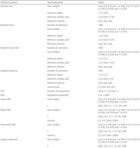
The reduced data set of 24 parameters is fitted using 9 distinct types of predictive models: logistic regression, linear discriminant analysis, quadratic discriminant ana-lysis, support vector machines (using linear, radial basis function and polynomial kernels), decision tree, random forest and stochastic gradient boosting. An exhaustive grid search is used based on 10-fold stratified cross-validation to determine the optimal hyper-parameters of each predictive model. The hyper-parameters that are optimized are presented in Table 1 with the optimal values in bold. The hyper-parameters that are not de-scribed in this table are set to the default values used in the scikit-learn library [27].
Logistic regression (LR) is a linear model that assumes that the targets follow a Gaussian distribution. A predic-tion on a transplantapredic-tion x is made using y(x) =wTx, wherewis the weight vector being learned.
Linear discriminant analysis (LDA) produces an opti-mally weighted linear function of chosen log-transformed markers and the discriminating threshold value minimizes the expected number of misclassifications under the nor-mal model.
Quadratic discriminant analysis (QDA) is related to LDA. Unlike LDA however, there is no assumption that the covariance of each class is identical. This produces a
quadratic discriminant function, which contains second order terms.
Support vector machines (SVMs) are sparse kernel machines, a type of models that rely only on a subset of the data (the support vectors) to predict unknown class labels. SVMs separate input data using a good-fitting hyperplane. Kernels can be used to transform this hyper-plane into a non-linear input separator. We chose a lin-ear, a radial basis function and a polynomial kernel.
A decision tree (DT) separates the data (the parent node) into two subsets (the child nodes) by the best splitting feature. The two resulting subsets become the new parent nodes, which are subsequently split further into two child nodes. This procedure continues until all observations are classified.
Random forest (RF) is an ensemble machine learning method based on the construction of multiple decision trees. The main underlying technique is bootstrap aggre-gating (bagging). In each decision tree, a data point falls into a particular leaf depending on its features and is assigned a prediction. The predictions of the data points are then averaged. RF has a built-in feature selection system and allows for joint features, making it not only an additive model but also a multiplicative one.
Stochastic gradient boosting (SGB) constructs additive regression tree models sequentially to fit pseudo-residuals of previous cumulative models. This stepwise manner combines the performance of weak learners (i.e., regres-sion trees here) iteratively into a strong learner with high accuracy.
As RF has a built-in feature selection system, the full data set of all collected parameters is also fitted using RF. By doing this, we can compare the performance between the RF fitted on the reduced data set and the RF fitted on the full data set, to evaluate if the recursive feature elimination procedure influences the built-in feature selection of RF.
Model validation
Performance of the models is assessed by computing the diagnostic test characteristics, including sensitivity and positive predictive value (PPV), and by evaluating the discriminative capacity, using the area under the receiver operating characteristic curve (AUROC), which mea-sures how well the relative ranking of the individual risk is in substantially the correct order (observed incidence in those with higher predicted risks are higher).
are used as training data. The cross-validation process is then repeated ten times, with each of the ten folds used exactly once as the validation data. The ten results from the folds are averaged to produce a single estimation. The advantage is that all observations are used for both training and validation, and each observation is used for validation exactly once.
Model comparison
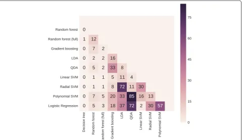
Subsequently, the models are pairwise compared. For each model, the AUROC is computed in each of the ten folds. The ten values for the AUROC of one model are compared with the values of another model using the two-sided Wilcoxon signed-rank test at 5 % significance level.
Table 1Optimal hyper-parameters after exhaustive grid search
Statistical method Hyper-parameter Values
Decision tree Class weights auto, 0 to 0.20 and 1 to 0.80, 0 to 0.10 and 1
to 0.90, 0 to 0.05 and 1 to 0.95
Maximum depth 1 to 10 (8)
Minimum samples split 2 to nVars+1 (18)
Maximum features auto, sqrt, log2
Random forest Number of estimators 1000
Class weights auto, 0 to 0.20 and 1 to 0.80, 0 to 0.10 and 1
to 0.90, 0 to 0.05 and 1 to 0.95
Maximum depth 1 to 10 (9)
Minimum samples split 2 to nVars+1 (24)
Maximum features auto, sqrt, log2
Random forest (full) Number of estimators 1000
Class weights auto, 0 to 0.20 and 1 to 0.80, 0 to 0.10 and 1
to 0.90, 0 to 0.05 and 1 to 0.95
Maximum depth 1 to 10 (1)
Minimum samples split 2 to nVars+1 (63)
Maximum features auto, sqrt, log2
Gradient boosting Number of estimators 1000
Maximum depth 1 to 10 (1)
Minimum samples split 2 to nVars+1 (9)
Maximum features auto, sqrt, log2
Learning rate 0.1, 0.05, 0.02, 0.01
LDA Number of components None or 1 to nVars +1
QDA Regularizing parameter 0 to 1 (0.89)
Linear SVM Class weights auto, 0 to 0.20 and 1 to 0.80, 0 to 0.10 and 1
to 0.90, 0 to 0.05 and 1 to 0.95
C 0.001, 0.01, 0.1, 1, 10, 100, 1000
Radial SVM Class weights auto, 0 to 0.20 and 1 to 0.80, 0 to 0.10 and 1
to 0.90, 0 to 0.05 and 1 to 0.95
C 0.001, 0.01, 0.1,1, 10, 100, 1000
Gamma 0.1, 0.01, 0.001, 0.0001
Polynomial SVM Class weights auto, 0 to 0.20 and 1 to 0.80, 0 to 0.10 and 1
to 0.90, 0 to 0.05 and 1 to 0.95
C 0.001, 0.01, 0.1,1, 10, 100, 1000
Gamma 0.1, 0.01, 0.001, 0.0001
Logistic regression Class weights auto, 0 to 0.20 and 1 to 0.80, 0 to 0.10 and 1
to 0.90, 0 to 0.05 and 1 to 0.95
C 0.001, 0.01, 0.1,1, 10, 100, 1000
All computations are carried out using Python, specific-ally in the SciPy environment using the scikit-learn library [27]. Continuous data are presented as mean ± standard deviation and categorical data are reported as percentages. Counts are put in parentheses.
Results
Descriptive statistics
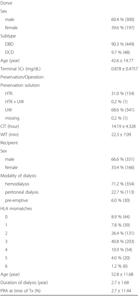
The most relevant donor, preservation/operation, and recipient characteristics are presented in Table 2. After exclusion, 497 transplantations are used for the analysis, consisting of 432 unique donors (362 donated a single kidney to a recipient of our center and the other kidney to a recipient of a different center, 5 donated both kid-neys to the same recipient of our center, and 65 donated both kidneys to different recipients of our center) and 496 unique recipients (1 recipient underwent two kidney transplantations at different times from deceased donors during the study period). The observed incidence of DGF is 12.5 % (62/497).
This imbalance in the data set is addressed by assigning more weight to the‘DGF’class during the learning phase of the predictive models. Only 11 (categorical) parameters out of the 55 retrospectively collected parameters are in-complete and contain missing values for a number of transplantations. The most frequent occurring value, which is the‘normal’category, is used to fill in these miss-ing values. This is a safe assumption, because‘abnormal’ values for risk factors are more likely to be emphasized and registered in the electronic medical records. However,
‘normal’values are not always routinely registered in the electronic medical records and are retrospectively consid-ered as missing values.
Model performance and comparison
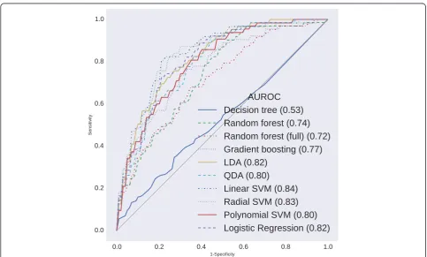
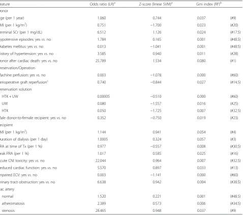
Diagnostic test characteristics and AUROCs after 10-fold stratified cross-validation are presented in Table 3. The re-ceiver operating characteristic curves and the p-values of the pairwise AUROC comparisons are presented in Figs. 1 and 2, respectively. The selected features and their respect-ive odds ratios (LR), Z-scores (linear SVM), and Gini index (RF fitted on the full data set) are presented in Table 4.
DT is not able to discriminate between recipients with and without DGF (AUROC of 52.5 %) and is inferior to the other methods.
As SGB and RF mainly have high sensitivity (98.8 and 96.3 %, respectively) and high PPVs (89.2 and 89.0 %, respectively) in identifying recipients without DGF, their discriminative capacity (AUROC of 77.2 and 73.9 %, re-spectively) is superior to DT. However, RF is still outper-formed by LDA, QDA, linear SVM, radial SVM and LR. SGB is only outperformed by linear SVM.
LDA and QDA already have higher sensitivity in identi-fying recipients with DGF (27.6 and 37.6 %, respectively)
and only slightly lower sensitivity in identifying recipients without DGF (94.7 and 89.9 %, respectively), resulting in higher discriminative capacity (AUROC of 82.2 and 79.6 %, respectively). Both LDA and QDA outperform DT and RF, but only QDA is inferior to linear SVM.
Amongst all methods used, linear SVM, radial SVM and LR have the highest sensitivity in identifying recipients with Table 2Baseline characteristics (n= 497)
Donor
Sex
male 60.4 % (300)
female 39.6 % (197)
Subtype
DBD 90.3 % (449)
DCD 9.7 % (48)
Age (year) 42.6 ± 14.77
Terminal SCr (mg/dL) 0.878 ± 0.4757
Preservation/Operation
Preservation solution
HTK 31.0 % (154)
HTK + UW 0.2 % (1)
UW 68.6 % (341)
missing 0.2 % (1)
CIT (hour) 14.19 ± 4.328
WIT (min) 22.3 ± 7.09
Recipient
Sex
male 66.6 % (331)
female 33.4 % (166)
Modality of dialysis
hemodialysis 71.2 % (354)
peritoneal dialysis 22.7 % (113)
pre-emptive 6.0 % (30)
HLA mismatches
0 8.9 % (44)
1 7.8 % (39)
2 26.4 % (131)
3 40.8 % (203)
4 10.9 % (54)
5 4.0 % (20)
6 1.2 % (6)
Age (year) 52.8 ± 11.68
Duration of dialysis (year) 2.7 ± 1.68
PRA at time of Tx (%) 2.7 ± 11.44
DGF (83.8, 88.8 and 85.5 %, respectively), at the expense of identifying recipients without DGF (72.0, 57.9 and 65.0 %, respectively). However, their capability to identify both out-comes is reflected in a strong discriminative capacity (AUROC of 84.3, 83.3 and 81.7 %, respectively). Linear SVM outperforms each method, except for radial SVM, polynomial SVM and LDA. Radial SVM and LR outper-form DT and RF, but only LR is inferior to linear SVM.
The performance of polynomial SVM is similar to that of SGB and RF, with high sensitivity (97.5 %) and high PPV (88.5 %) in identifying recipients without DGF, resulting in an AUROC of 79.8 %. Polynomial SVM also outperforms DT. Unlike SGB and RF however, it is not inferior to any of the methods used.
RF fitted on the full data set has a sensitivity of 100 % and a PPV of 87.5 % in identifying recipients without Table 3Performance of the statistical methods after 10-fold stratified cross-validation
Statistical method Sensitivity (%) PPV (%) AUROC (%)
No DGF DGF No DGF DGF
Decision tree 75.4 ± 6.64 29.5 ± 16.29 88.2 ± 2.73 14.2 ± 8.13 52.5 ± 8.55
Gradient boosting 98.8 ± 1.55 16.2 ± 12.94 89.2 ± 1.67 58.3 ± 38.19 77.2 ± 9.64
Random forest 96.3 ± 4.05 16.4 ± 14.92 89.0 ± 2.09 43.9 ± 38.19 73.9 ± 9.94
Random forest (full) 100.0 ± 0.00 0.0 ± 0.00 87.5 ± 0.64 0.0 ± 0.00 71.6 ± 12.38
LDA 94.7 ± 2.92 27.6 ± 15.10 90.2 ± 2.00 42.3 ± 19.94 82.2 ± 6.14
QDA 89.9 ± 5.35 37.6 ± 17.26 91.0 ± 2.55 37.9 ± 20.82 79.6 ± 7.55
Linear SVM 72.0 ± 6.29 83.8 ± 7.51 96.9 ± 1.34 30.6 ± 5.60 84.3 ± 4.11
Radial SVM 57.9 ± 7.45 88.8 ± 7.38 97.2 ± 1.87 23.6 ± 4.14 83.3 ± 4.05
Polynomial SVM 97.5 ± 1.90 10.9 ± 12.20 88.5 ± 1.14 24.0 ± 24.17 79.8 ± 5.33
Logistic regression 65.0 ± 8.25 85.5 ± 8.94 96.9 ± 1.84 26.5 ± 4.75 81.7 ± 5.82
Abbreviations:AUROCarea under the receiver operating characteristic curve,DGFdelayed graft function,LDAlinear discriminant analysis,PPVpositive predictive value,QDAquadratic discriminant analysis,SVMsupport vector machine
DGF, resulting in an AUROC of 71.6 %. It is superior to DT, which is fitted on the reduced data set and has no discriminative capacity, and non-inferior to RF fitted on the reduced data set. However, RF fitted on the full data set is inferior to each of the other methods used.
Discussion
The risk prediction of DGF may be important in pre-venting its deleterious short-term and long-term conse-quences. To date, four predictive models are developed as a clinical tool to quantify the risk for DGF [14–17]. All models are developed using LR. We compared in this study several machine learning methods, including LR, in terms of their predictive accuracy for DGF. There are no studies that have used DT, SGB, RF, LDA, QDA or SVM in the prediction of DGF.
In our study, DT is not able to discriminate between recipients with and without DGF, and is inferior to the other methods. SGB, RF and polynomial SVM are mainly able to identify recipients without DGF and only outperform DT. Despite lower sensitivity in varying degrees to identify recipients without DGF, LDA, QDA, radial SVM and LR also have the ability to identify recipients with DGF, resulting in higher discriminative capacity, which outperforms DT and RF. Linear SVM has the highest discriminative capacity (AUROC of 84.3 %), outperforming each method, except for radial
SVM, polynomial SVM and LDA. However, it is the only method superior to LR.
The AUROC focuses solely on the predictive accuracy of a model. As such, it cannot tell us whether the model is worth using in clinical practice, because it does not in-corporate information on consequences. The method with maximal accuracy is not necessarily the best to choose. This choice should depend on the disadvantages or costs of not identifying a recipient with DGF as op-posed to incorrectly predicting DGF in a recipient who will not develop it [28]. The advantages of an early hypo-thetic treatment should be weighed against possible iat-rogenic damage and unnecessary additional costs. If we assume that the damage of an unnecessary treatment of DGF (a false-positive result) is limited, a more sensitive method should be used. If an unnecessary treatment is harmful, a more specific method should be used. Of course the trade-off between sensitivity and specificity should be kept in mind: a very sensitive method is use-less when it is not specific enough and vice versa [29].
potential benefit of an early management, because DGF has deleterious short-term and long-term consequences. To date, a more sensitive method is therefore preferred. In our study, linear SVM, radial SVM and LR have the high-est sensitivity in identifying recipients with DGF (83.8, 88.8 and 85.5 %, respectively).
To sum up, the discriminative capacities of LDA, linear SVM, radial SVM and LR are the only ones above 80 % (82.2, 84.3, 83.3 and 81.7 %, respectively). None of the pairwise AUROC comparisons between these models is statistically significant, except linear SVM outperforming LR. Additionally, a method with higher sensitivity is preferred over a method with higher specificity in the
prediction of DGF. The sensitivity of linear SVM to iden-tify recipients with DGF (83.8 %) is amongst the three highest of all methods used. Only radial SVM and LR have a slightly higher sensitivity (88.8 and 85.5 %, respectively). Due to both reasons, the authors believe that linear SVM is most appropriate to predict DGF.
72.0 % of the recipients who will not develop DGF are identified. These recipients can undergo the kidney trans-plantation without the need for a more precise monitor-ing. Only 3.1 % will still develop DGF. 83.8 % of the recipients who will develop DGF are identified. These re-cipients will have to be precisely monitored after kidney transplantation, making an early identification of graft Table 4Weights of the selected features
Feature Odds ratio (LR)a Z-score (linear SVM)a Gini index (RF)b
Donor
Age (per 1 year) 1.060 0.744 0.037 (#9)
BMI (per 1 kg/m2) 0.751 −1.700 0.023 (#20)
Terminal SCr (per 1 mg/dL) 6.512 1.126 0.024 (#17.5)
Hypotensive episodes: yesvs.no 1.784 0.165 0.001 (#48.5)
Diabetes mellitus: yesvs.no 0.013 −1.041 0.001 (#48.5)
History of hypertension: yesvs.no 3.585 0.940 0.011 (#28)
Donor after cardiac death: yesvs.no 25.789 1.534 0.080 (#1)
Preservation/Operation
Machine perfusion: yesvs.no 0.003 −1.078 0.000 (#60)
Perioperative graft reperfusionc 0.740 −0.844 0.027 (#14.5)
Preservation solution
HTK + UW 0.00005 −0.510 0.000 (#60)
UW 0.080 −1.557 0.016 (#25)
HTK 0.050 −1.725 0.007 (#32.5)
Male donor-to-female recipient: yesvs.no 0.352 −0.750 0.019 (#23)
Recipient
BMI (per 1 kg/m2) 1.144 0.941 0.054 (#4)
Duration of dialysis (per 1 day) 1.0005 0.324 0.057 (#3)
PRA at time of Tx (per 1 %) 0.977 −0.557 0.008 (#30.5)
Peak PRA (per 1 %) 1.017 0.585 0.025 (#16)
Acute CNI toxicity: yesvs.no 22.044 0.964 0.007 (#32.5)
Reduced cardiac function: yesvs.no 5.570 0.897 0.033 (#13)
Impaired ECV: yesvs.no 0.003 −1.141 0.000 (#60)
Urinary tract obstruction: yesvs.no 6.638 0.942 0.004 (#38.5)
Iliac artery
normal 1.520 0.221 0.001 (#48.5)
atheromatosis 2.389 0.573 0.006 (#34.5)
stenosis 28.465 0.948 0.037 (#9)
a
Fitted on the reduced data set b
Fitted on the full data set. Tied rank amongst all 68 features is given in parentheses c
Perioperative graft reperfusion is an ordinal feature (poor–patchy–moderate–good)
dysfunction possible. 69.4 % of all positively identified re-cipients will eventually not develop DGF.
Our study does have limitations. Firstly, our sample size of approximately 500 transplantations is lower than in the existing models. It is known that machine learning tech-niques generally benefit from a large amount of data, in-creasing their performance [19]. However, we benefited from the detailed and high-quality peritransplant data that could be collected, which is largely unavailable in regis-tries. Secondly, the incidence of DGF in our cohort is lower than in the existing models. This imbalance is ad-dressed by assigning more weight to the‘DGF’class dur-ing the learndur-ing phase of the predictive models. Thirdly, single-center models limit generalizability. However, we used cross-validation to attenuate the generalization error. Finally, our analysis included most, but not all, of the identified risk factors for DGF.
Conclusions
Nine distinct types of predictive models for DGF are considered. The discriminative capacities of LDA, linear SVM, radial SVM and LR are the only ones above 80 %. None of the pairwise AUROC comparisons between these models is statistically significant, except linear SVM outperforming LR. Additionally, a method with higher sensitivity is preferred over a method with higher specificity in the prediction of DGF, because the damage of an unnecessary biopsy is outweighed by the potential benefit of an early management. The sensitivity of linear SVM to identify recipients with DGF is amongst the three highest of all models. Due to both reasons, the authors believe that linear SVM is most appropriate to predict DGF.
Abbreviations
AUROC:Area under the receiver operating characteristic curve; DGF: Delayed graft function; DT: Decision tree; LDA: Linear discriminant analysis; LR: Logistic regression; PPV: Positive predictive value; QDA: Quadratic discriminant analysis; RF: Random forest; SGB: Stochastic gradient boosting; SVM: Support vector machine.
Competing interests
The authors declare that they have no competing interests.
Authors’contributions
AD and PD designed study, collected data, interpreted statistical analysis and drafted paper. Both authors contributed equally to this study and are the joint first authors. PP, FV and TD designed study and revised paper. IC designed study, performed and interpreted statistical analysis, and revised paper. All authors read and approved the final manuscript.
Authors’information
Alexander Decruyenaere and Philippe Decruyenaere are the joint first authors.
Acknowledgements
The authors would like to thank the transplant coordinators, with special thanks to Marc Van Der Vennet, for providing part of the data. The authors declare that they have not received any funding.
Author details 1
Department of Nephrology, Ghent University Hospital, Ghent, Belgium. 2Department of Thoracic and Vascular Surgery, Ghent University Hospital,
Ghent, Belgium.3Department of Information Technology (INTEC), Ghent University - iMinds, Ghent, Belgium.
Received: 16 April 2015 Accepted: 30 September 2015
References
1. Purnell TS, Auguste P, Crews DC, Lamprea-Montealegre J, Olufade T, Greer R, et al. Comparison of life participation activities among adults treated by hemodialysis, peritoneal dialysis, and kidney transplantation: a systematic review. Am J Kidney Dis. 2013;62(5):953–73.
2. Tonelli M, Wiebe N, Knoll G, Bello A, Browne S, Jadhav D, et al. Systematic review: kidney transplantation compared with dialysis in clinically relevant outcomes. Am J Transplant. 2011;11(10):2093–109.
3. Cavaille-Coll M, Bala S, Velidedeoglu E, Hernandez A, Archdeacon P, Gonzalez G, et al. Summary of FDA workshop on ischemia reperfusion injury in kidney transplantation. Am J Transplant. 2013;13(5):1134–48.
4. Yarlagadda SG, Coca SG, Garg AX, Doshi M, Poggio E, Marcus RJ, et al. Marked variation in the definition and diagnosis of delayed graft function: a systematic review. Nephrol Dial Transplant. 2008;23(9):2995–3003. 5. Sharif A, Borrows R. Delayed graft function after kidney transplantation: the
clinical perspective. Am J Kidney Dis. 2013;62(1):150–8.
6. Siedlecki A, Irish W, Brennan DC. Delayed graft function in the kidney transplant. Am J Transplant. 2011;11(11):2279–96.
7. Perico N, Cattaneo D, Sayegh MH, Remuzzi G. Delayed graft function in kidney transplantation. Lancet. 2004;364(9447):1814–27.
8. Matas AJ, Gillingham KJ, Elick BA, Dunn DL, Gruessner RW, Payne WD, et al. Risk factors for prolonged hospitalization after kidney transplants. Clin Transpl. 1997;11(4):259–64.
9. Rosenthal JT, Danovitch GM, Wilkinson A, Ettenger RB. The high cost of delayed graft function in cadaveric renal transplantation. Transplantation. 1991;51(5):1115–8.
10. Yarlagadda SG, Coca SG, Formica Jr RN, Poggio ED, Parikh CR. Association between delayed graft function and allograft and patient survival: a systematic review and meta-analysis. Nephrol Dial Transplant. 2009;24(3):1039–47.
11. Shoskes DA, Cecka JM. Deleterious effects of delayed graft function in cadaveric renal transplant recipients independent of acute rejection. Transplantation. 1998;66(12):1697–701.
12. Troppmann C, Gruessner AC, Gillingham KJ, Sutherland DE, Matas AJ, Gruessner RW. Impact of delayed function on long-term graft survival after solid organ transplantation. Transplant Proc. 1999;31(1–2):1290–2. 13. Tapiawala SN, Tinckam KJ, Cardella CJ, Schiff J, Cattran DC, Cole EH, et al.
Delayed graft function and the risk for death with a functioning graft. J Am Soc Nephrol. 2010;21(1):153–61.
14. Jeldres C, Cardinal H, Duclos A, Shariat SF, Suardi N, Capitanio U, et al. Prediction of delayed graft function after renal transplantation. Can Urol Assoc J. 2009;3(5):377–82.
15. Irish WD, Ilsley JN, Schnitzler MA, Feng S, Brennan DC. A risk prediction model for delayed graft function in the current era of deceased donor renal transplantation. Am J Transplant. 2010;10(10):2279–86.
16. Chapal M, Le Borgne F, Legendre C, Kreis H, Mourad G, Garrigue V, et al. A useful scoring system for the prediction and management of delayed graft function following kidney transplantation from cadaveric donors. Kidney Int. 2014;86(6):1130–9.
17. Zaza G, Ferraro PM, Tessari G, Sandrini S, Scolari MP, Capelli I, et al. Predictive model for delayed graft function based on easily available pre-renal transplant variables. Intern Emerg Med. 2015;10(2):135–41. 18. Greco R, Papalia T, Lofaro D, Maestripieri S, Mancuso D, Bonofiglio R.
Decisional trees in renal transplant follow-up. Transplant Proc. 2010;42(4):1134–6.
19. Lasserre J, Arnold S, Vingron M, Reinke P, Hinrichs C. Predicting the outcome of renal transplantation. J Am Med Inform Assoc. 2012;19(2):255–62.
20. Brier ME, Ray PC, Klein JB. Prediction of delayed renal allograft function using an artificial neural network. Nephrol Dial Transplant. 2003;18(12):2655–9. 21. Santori G, Fontana I, Valente U. Application of an artificial neural network
22. Akl A, Ismail AM, Ghoneim M. Prediction of graft survival of living-donor kidney transplantation: nomograms or artificial neural networks? Transplantation. 2008;86(10):1401–6.
23. Goldfarb-Rumyantzev AS, Scandling JD, Pappas L, Smout RJ, Horn S. Prediction of 3-yr cadaveric graft survival based on pre-transplant variables in a large national dataset. Clin Transpl. 2003;17(6):485–97.
24. Krikov S, Khan A, Baird BC, Barenbaum LL, Leviatov A, Koford JK, et al. Predicting kidney transplant survival using tree-based modeling. ASAIO J. 2007;53(5):592–600.
25. Brown TS, Elster EA, Stevens K, Graybill JC, Gillern S, Phinney S, et al. Bayesian modeling of pretransplant variables accurately predicts kidney graft survival. Am J Nephrol. 2012;36(6):561–9.
26. Guyon I, Weston J, Barnhill S, Vapnik V. Gene selection for cancer classification using support vector machines. Mach Learn. 2002;46(1–3):389–422. 27. Pedregosa F, Varoquaux G, Gramfort A, Michel V, Thirion B, Grisel O, et al.
Scikit-learn: machine learning in python. J Mach Learn Res. 2011;12:2825–30. 28. Vickers AJ, Elkin EB. Decision curve analysis: a novel method for evaluating
prediction models. Med Decis Making. 2006;26(6):565–74. 29. Zweig MH, Campbell G. Receiver-operating characteristic (ROC) plots: a
fundamental evaluation tool in clinical medicine. Clin Chem. 1993;39(4):561–77. 30. Powell JT, Tsapepas DS, Martin ST, Hardy MA, Ratner LE. Managing renal
transplant ischemia reperfusion injury: novel therapies in the pipeline. Clin Transpl. 2013;27(4):484–91.
Submit your next manuscript to BioMed Central and take full advantage of:
• Convenient online submission
• Thorough peer review
• No space constraints or color figure charges
• Immediate publication on acceptance
• Inclusion in PubMed, CAS, Scopus and Google Scholar
• Research which is freely available for redistribution